PI Tank Calculations

This document investigates the theory behind the PI-tank, which is a subject dating back more than a century. The challenge is to find a working design that is understandable. Most amateur solutions consist of tables or equations without explanation. Some on-line calculators refer to equations stated in historic documents. However, I have an aversion to using equations without understanding derivation and without knowing the source. The purpose of this document is to investigate the derivation of the equations and check them against other sources.

The Problem

The following diagram is a simple PI arrangement. The approach is to use complex analysis to find the impedance looking into the network Zin. The first stage is to combine C2 and R as a parallel circuit. The next stage is to add L in series and then convert L, C2 and R into an equivalent parallel network. It should be possible to find the dynamic impedance of the parallel circuit for a given Q.

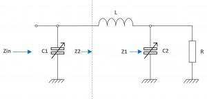
The wanted impedance at the input is Rp

Derivation of the above equations

Taking C2 and R in parallel, the combined impedance is the product over sum:

$Z_{1}=\frac{\dfrac{R}{j\omega C_{2}}}{R+\cfrac{1}{j\omega C_{2}}}=\cfrac{R}{1+j\omega C_{2}R} \hspace{2.5cm}\text{Equation 1}$

Taking into account the series impedance due to ‘L’:

$Z_{2}=j\omega L+\dfrac{R}{1+j\omega C_{2}R} \hspace{3.7cm}\text{Equation 2}$

Convert this into a series circuit by multiplying the second term top and bottom by the complex conjugate. This removes the ‘j’ terms in the denominator:

$Z_{2}=j\omega L+\dfrac{R}{1+j\omega C_{2}R}\left ( \dfrac{1-j\omega C_{2}R}{1-j\omega C_{2}R} \right )$

After multiplying out:

$Z_{2}=j\omega L+\dfrac{R}{1+\omega^2 C_{2}^2R^2}-\dfrac{j\omega C_{2}R^2}{1+\omega^2 C_{2}^2R^2}$

After tidying up:

$Z_{2}=\dfrac{R}{1+\omega^2 C_{2}^2R^2}+j\left (\omega L-\frac{\omega C_{2}R^2}{1+\omega^2 C_{2}^2R^2} \right ) \hspace{1.5cm} \text{Equation 3}$

Comparing Equation 3 against the standard series complex impedance:

$Z_{2}=R_{s}+jX_{s}$

Hence:

$R_{s}=\dfrac{R}{1+\omega^2 C_{2}^2R^2} \hspace{1.0cm}and \hspace{1.0cm} X_{s}=\left (\omega L-\frac{\omega C_{2}R^2}{1+\omega^2 C_{2}^2R^2} \right )$

In a series circuit, the circuit Q is defined as the ratio of reactance to resistance. Some texts complicate the issue by referring to loaded and unloaded Q. Here, Q is assumed to be the loaded Q which is the Q of the tank circuit with the load R connected (This is 50Ω in this case). An assumption is made that the coil and capacitor is constructed from low loss components and that the unloaded Q (The Q without R connected) is much higher than the loaded Q.

Hence the value of Q is:

$Q=\frac{X_{s}}{R_{s}}$

After substituting:

$Q=\dfrac{\omega L-\dfrac{\omega C_{2}R^2}{1+\omega^2 C_{2}^2R^2}}{\dfrac{R}{1+\omega^2 C_{2}^2R^2}}=\dfrac{\omega L\left ( 1+\omega^2 C_{2}^2R^2 \right )}{R}-\omega C_{2}R \hspace{1.5cm} \text{Equation 4}$

Equation 4 is needed later.

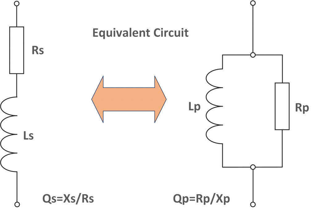
The next stage is to convert the series circuit, Equation 3, into a parallel circuit. When converted, the result will be a parallel resistance known as the dynamic impedance in parallel with an inductive reactance. The capacitor C1 is then placed in parallel and is used to tune the inductance to resonance.

The next stage is converting Equation 3 into an equivalent parallel equivalent circuit using the following equations. The subscript ‘s’ means ‘series’ and ‘p’ means ‘parallel’. These results are derived in the appendix to this document.

$R_{p}=R_{s}\left ( 1+Q^2 \right )\hspace{3.0cm} \hspace{0.1cm} \text{Equation A5 - See Appendix A of this document}$

and

$X_{p}=X_{s}\left ( 1+\dfrac{1}{Q^2} \right ) \hspace{2.5cm} \text{Equation A6 - See Appendix A of this document}$

Hence, substituting for the series components:

$R_{p}=\dfrac{R}{1+\omega^2 C_{2}^2R^2}\left ( 1+Q^2 \right ) \hspace{4cm} \text{Equation 5}$

and

$X_{p}=\left (\omega L-\frac{\omega C_{2}R^2}{1+\omega^2 C_{2}^2R^2} \right )\left ( 1+\dfrac{1}{Q^2} \right ) \hspace{2cm}\text{Equation 6}$

Rearrange Equation 5 to give:

$1+\omega^2 C_{2}^2R^2=\frac{R}{R_{p}}\left ( 1+Q^2 \right ) \hspace{4.0cm} \text{Equation 7}$

Also, from Equation 7:

$\omega C_{2}R=\pm \sqrt{\frac{R}{R_{p}}\left ( 1+Q^2 \right )-1} \hspace{3.8cm} \text{Equation 8}$

Strictly speaking the square root is plus or minus. However, the correct sign in this application is positive. Now substitute Equation 7 into Equation 4:

$Q=\dfrac{\omega L\left ( 1+Q^2 \right )}{R_{p}}-\omega C_{2}R \hspace{4.4cm} \text{Equation 9}$

Substitute Equation 8 into Equation 9:

$Q=\dfrac{\omega L\left ( 1+Q^2 \right )}{R_{p}}-\sqrt{\frac{R}{R_{p}}\left ( 1+Q^2 \right )-1} \hspace{2.2cm} \text{Equation 10}$

Equation 10 is now solved for L:

Notes

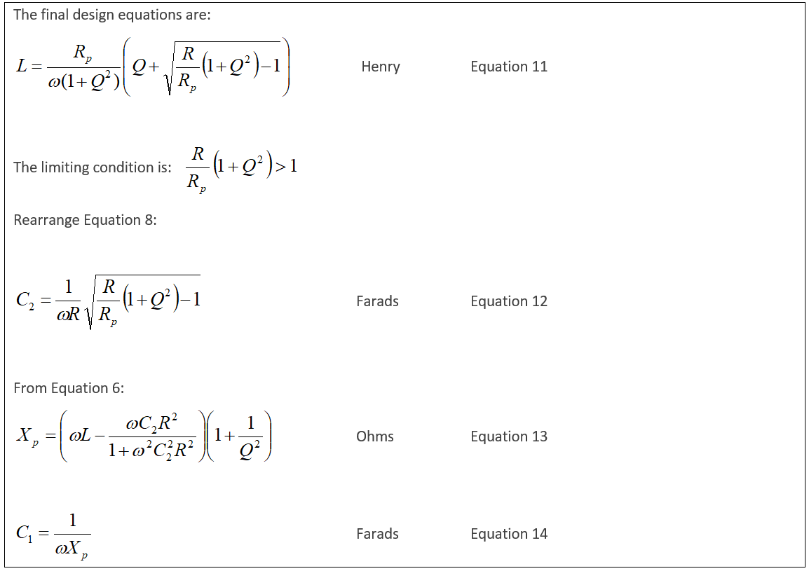
• In equation 11, the only terms are the anode load impedance Rp, L, R and the circuit Q.

• The value of equation 12 does not depend upon L.

• The capacitor C1 is only required to tune out the inductive reactance which then completes the match. This is probably why, for the last 100 years, the capacitor C2 has been called the load capacitor and why C1 has been called the tune capacitor!

Practical Example

To provide an example, Figure 1 shows a MathCad worksheet for 2MHz, a Q of 11, a load of 50Ω and a target anode load impedance of 5000Ω. It is best to calculate the parameters in the order: equations 11, 12, 13 and then 14. The Mathcad sheet is WYSIWYG and calculates the formulas numerically as shown below. The phase plot shows that, at resonance, the impedance looking into the PI-tank is indeed 5000Ω resistive.

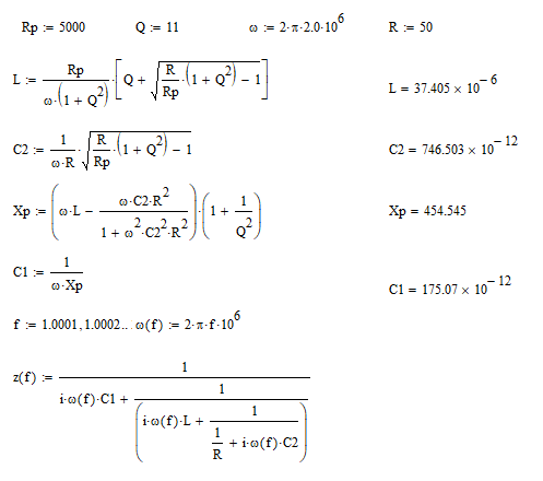
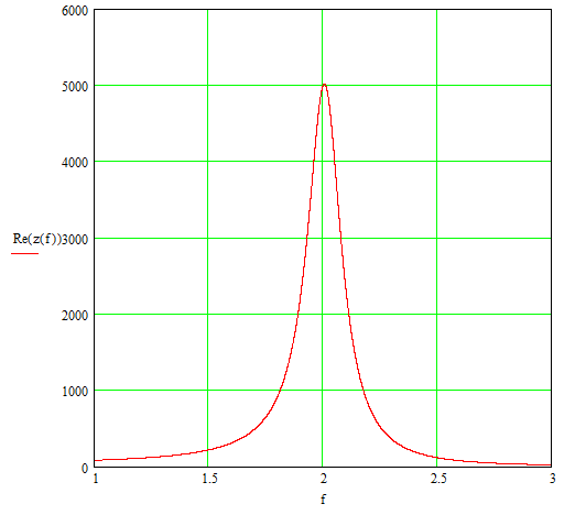
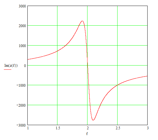
Figure 1 – Pi-Tank Impedance Measured against Frequency (MHz) – Example

Very often, we need to calculate C1, C2 and the associated Q for a given inductor value. This happens when a practical coil is wound and the resulting inductance is close to the idea value but not exact. In this case, you will need to know if the tank will tune without having to actually try it for real. Rearranging equation 10 gives the Q:

$Q=\dfrac{R_{p}+\sqrt{RR_{p}-L^2\omega ^2}}{\omega L} \hspace{2.2cm} \text{Equation 15}$

This rearrangement is quite tricky to calculate. Q ends up as a quadratic equation with two solutions. The above is the correct version. The derivation of this equation is provided in Appendix B. Equation 15 is used to calculate the Q before evaluating equations 12, 13 and 14 to determine the other parameters. The components are assumed ideal.

Comparison with other Calculators and Designs

An objective of this document is to compare the values predicted by equations 11, 12, 13 and 14 against other designs and on line calculators. For this comparison I assumed an anode impedance of 5000Ω to allow comparison against the G2DAF design. I included amateur bands all the way down to 475kHz.

The load is assumed 50Ω, anode load 5000Ω the Q is assumed 12.

Band	Element	This Document	On Line Calculator Note 1	On Line Calculator Note 2	G2DAF Note 3	ARRL Handbook 1983 Note 4
0.475 MHz	C1	804.1 pF	804 pF	804.1 pF
	L	146.4 μH	146 μH	146.4 μH
	C2	4495 pF	4500 pF	4495.3 pF
1.9 MHz	C1	201 pF	201 pF	201 pF
	L	36.6 μH	36.6 μH	36.6 μH
	C2	1124 pF	1120 pF	1123.8 pF
3.7 MHz	C1	103.2 pF	103 pF	103.2 pF	116 pF	118 pF
	L	18.8 μH	18.8 μH	18.8 μH	20 μH	18.6 μH
	C2	577.1 pF	577 pF	577.1 pF	900 pF	766 pF
7.1 MHz	C1	53.8 pF	53.8 pF	53.8 pF	58 pF	59 pF
	L	9.8 μH	9.8 μH	9.8 μH	10 μH	9.28 μH
	C2	300.7 pF	301 pF	300.7 pF	450 pF	383 pF
14.2 MHz	C1	26.9 pF	26.9 pF	26.9 pF	29 pF	30 pF
	L	4.9 μH	4.9 μH	4.9 μH	5 μH	4.6 μH
	C2	150.3 pF	150 pF	150.4 pF	225 pF	192 pF
21.2 MHz	C1	18.0 pF	18 pF	18 pF	20 pF	20 pF
	L	3.3 μH	3.3 μH	3.3 μH	3.5 μH	3.1 μH
	C2	100.7 pF	101 pF	100.7 pF	160 pF	128 pF
29 MHz	C1	13.2 pF	13.2 pF	13.1 pF	15 pF	15 pF
	L	2.4 μH	2.4 μH	2.4 μH	2.5 μH	2.32 μH
	C2	73.6 pF	73.6 pF	73.6 pF	113 pF	96 pF

Note 1: This is taken from the excellent OwenDuffy.net site that presents an on-line calculator based on the Eimac “Care and Feeding of Power Grid Tubes 5th edition 2003” book. On inspection, the equations presented in the Eimac document turn out to be (essentially) identical to the equations derived here. There are some differences in appearance but these can be shown identical by suitable substitutions. The results are identical. https://owenduffy.net/calc/pi.htm

Note 2: https://www.changpuak.ch/electronics/calc_18.php The web site does not state the equations or the source of the equations but the results are the same numerically. I suspect the calculator uses the same source as the OwenDuffy.net calculator.

Note 3: The document by G2DAF states that the method of calculating the PI tank components is an approximation. Surprisingly, the results are similar particularly the inductors. With variable capacitors, the tank circuits would be perfectly acceptable. Note that the G2DAF results were calculated for a Q of 12 and output impedance of 75Ω and not 50Ω.

Note 4: This data is presented as a table for Q=12 only. Note the frequencies are approximate. No explanation for the data or derivation were given. Later, in the 1997 ARRL handbook, the method of calculation changed and equations are quoted. Unfortunately, the tables now only covered loads from 1500Ω to 2500Ω. The 1997 book provided software to calculate other values.

Conclusion

Metaphorically speaking, I have reinvented the wheel and taught grandma how to suck eggs. Most of the existing calculations provide perfectly satisfactory results. For me it has been an interesting investigation and I now understand the PI-tank a little better. The only limitation I can see in these calculations is the condition:

$\frac{R}{R_{p}}\left ( 1+Q^2 \right )>1$

If you attempt a large impedance transformation, the loaded Q must be sufficient. For example, transforming 50Ω to 5000Ω, the Q must be 9.95 or greater. If you try to calculate results for lower Q, then C1 and C2 become complex which is nonsense.

I conclude that the OwenDuffy.net site provides identical results and involves no approximations. I recommend using that site with confidence.

Appendix A – Convert a Series Impedance to an Equivalent Parallel Circuit

This appendix demonstrates how to convert from a series to a parallel tuned circuit of known Q.

The circuit Q is identical in both arrangements because the circuits are equivalent. In the above example, the reactance is inductive but expressions can easily be calculated for capacitive reactance (not done here).

First, find the parallel impedance by taking the product over sum and then multiply top and bottom by the conjugate of the denominator:

$Z_{p}=\dfrac{j\omega L_{p}R_{p}}{R_{p}+j\omega L_{p} }=\dfrac{j\omega L_{p}R_{p}}{R_{p}+j\omega L_{p} }\left (\frac{R_{p}-j\omega L_{p} }{R_{p}-j\omega L_{p} } \right )$

Express this in series form:

$Z_{p}=\dfrac{\omega ^2 L_{p}^2 R_{p}}{R_{p}^2+\omega^2 L_{p}^2 } +\dfrac{j\omega L_{p}R_{p}^2 }{R_{p}^2+\omega^2 L_{p}^2 }$

Here, the equivalent series impedance takes the form:

$Z_{p}=R_{s}+j\omega L_{s}$

$R_{s}=R_{p}\left (\dfrac{\omega ^2 L_{p}^2 }{R_{p}^2+\omega^2 L_{p}^2 } \right )\hspace{3.9cm} \text{Equation A1}$

$L_{s}=L_{p}\left ( \dfrac{R_{p}^2 }{R_{p}^2+\omega^2 L_{p}^2 } \right )\hspace{4.0cm} \text{Equation A2}$

However, for a parallel connection, Q is defined as the parallel resistance divided by the reactance:

$Q=Q_{p}=\frac{R_{p}}{\omega L_{p}}$

So, rearranging equations A1 and A2:

$R_{s}=R_{p}\left ( \frac{1}{1+Q^2} \right ) \hspace{4.0cm} \text{Equation A3}$

$L_{s}=L_{p}\left ( \dfrac{1}{1+\dfrac{1}{Q^2}} \right )\hspace{3.8cm} \text{Equation A3}$

To convert in the other direction from series to parallel, rearrange equations A3 and A4:

$R_{p}=R_{s}\left ( 1+Q^2 \right )\hspace{4.3cm} \text{Equation A5}$

$L_{p}=L_{s}\left ( 1+\dfrac{1}{Q^2} \right )\hspace{4.0cm} \text{Equation A6}$

==========================================

Some engineers avoid using secondary parameters such as Q because it can cause confusion. In this case, Q removes unnecessary complexity and is quite useful.

End of Appendix A

Appendix B – Convert Equation 10 into Equation 15

This is quite tricky and took several attempts so I recorded the arithmetic for posterity. The task is to express equation 10 making Q the subject:

$Q=\dfrac{\omega L\left ( 1+Q^2 \right )}{R_{p}}-\sqrt{\frac{R}{R_{p}}\left ( 1+Q^2 \right )-1} \hspace{2.2cm} \text{Equation 10}$

First eliminate the square root by rearranging and then squaring both sides:

$\left (\sqrt{\frac{R}{R_{p}}\left ( 1+Q^2 \right )-1} \right )^2=\left (\dfrac{\omega L\left ( 1+Q^2 \right )}{R_{p}}-Q \right) \left (\dfrac{\omega L\left ( 1+Q^2 \right )}{R_{p}}-Q\right)$

Multiply out and add 1 to each side:

$\frac{R}{R_{p}}\left ( 1+Q^2 \right )=\dfrac{\omega^2 L^2\left ( 1+Q^2 \right )^2}{R_{p}^2}-2Q\dfrac{\omega L\left ( 1+Q^2 \right )}{R_{p}}+\left ( 1+Q^2 \right )$

divide through by:

$\left ( 1+Q^2 \right )$

giving:

$\frac{R}{R_{p}}=\dfrac{\omega^2 L^2\left ( 1+Q^2 \right )}{R_{p}^2}-2Q\dfrac{\omega L}{R_{p}}+1$

Arrange as a quadratic in Q:

$\frac{\omega ^2L^2Q^2}{R_{p}^2}-2Q\dfrac{\omega L}{R_{p}}+\left ( 1+\frac{\omega ^2L^2}{R_{p}^2}-\frac{R}{R_{p}} \right )=0$

Divide through by:

$\dfrac{\omega ^2L^2}{R_{p}^2 }$

To give:

$Q^2-2Q\frac{\omega L}{R_{p}}\frac{R_{p}^2}{\omega ^2L^2}+\left ( \frac{R_{p}^2}{\omega ^2L^2}+\frac{\omega ^2L^2}{R_{p}^2}\frac{R_{p}^2}{\omega ^2L^2}-\frac{R}{R_{p}}\frac{R_{p}^2}{\omega ^2L^2} \right )=0$

Tidy up

$Q^2-\frac{\2R_{p}}{\omega L}Q+\left ( \frac{R_{p}^2}{\omega ^2L^2}+1-\frac{RR_{p}}{\omega ^2L^2} \right )=0$

Using the quadratic formula:

$Q=\frac{1}{2}\frac{2R_{p}}{\omega L}\pm \frac{1}{2}\sqrt{\frac{4R_{p}^2}{\omega ^2L^2}-4\left ( \frac{R_{p}^2}{\omega ^2L^2}+1 -\frac{RR_{p}}{\omega ^2L^2} \right )}$

$Q=\frac{R_{p}}{\omega L}\pm \sqrt{\frac{RR_{p}}{\omega ^2L^2}-1}$

Hence, taking the positive option (this is the one that works – found by trial and error)

$Q=\dfrac{R_{p}+\sqrt{RR_{p}-L^2\omega ^2}}{\omega L} \hspace{2.2cm} \text{Equation 15}$

Sorry that was so tedious!

73 Chris