Causality – Why Inductors are lossy

Overview

Causality is important. It impacts radio experiments in subtle ways – it introduces unexpected loss – don’t ignore it.

Causality is the condition forcing the output of a circuit to appear after connection of the input signal. A non-causal circuit creates an output before the input is connected that, effectively, sends energy into the past or future! This can happen in mathematical models but mother nature guarantees that it does not happen in the ‘real world’. As a consequence, certain relationships must exist that creates unexpected effects.

This document investigates causality and the relationship between the real and imaginary parts of the transfer function in a circuit. The circuit could be anything: an antenna, network or a loading coil.

Uncertainty of RF Components

Causality complicates RF engineering and causes confusion. For example, if you wind an inductor, either on a ferrite ring or on an air-spaced former, the resulting inductance will vary with frequency and a frequency dependent series resistance will unexpectedly ‘appear’. For example, an online calculator reported that 16 turns wound on an FT50-43 core generated about 112.64 μH at 1 MHz.

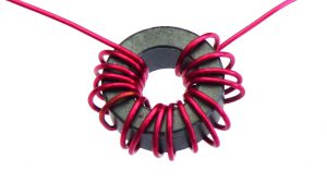
Figure 1 – FT50-43 Core with 16 Turns

It also reported that at 30 MHz, the inductance remained the same at 112.64 μH. However, a real FT50-43 core measured on the bench demonstrated the following plot:

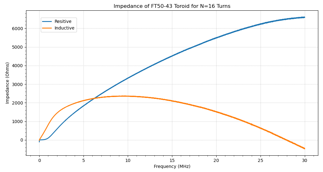
Figure 2 – Frequency-Domain Measurement of Real and Imaginary Series Impedance

At 1 MHz the network analyser reported 134 μH (More or less as expected). At 30 MHz, the inductor behaves like a capacitor. The series resistive component exceeded 1 kΩ over most of the range and exceeded 6 kΩ at 30 MHz. Just where did that come from? What mechanism inserts 6 kΩ into an inductor?

At 27.95 MHz the inductive reactance falls to zero and the coil behaves like a pure 6.4 kΩ resistor! It seems like magic – no wonder RF engineering is so mysterious.

As a side note: if you use the same FT50-43 core with 16 turns, as above, and then wind another winding with 16 turns and use it as a transformer, the 6 kΩ coil resistance suddenly and conveniently disappears! Where did it go? You end up with a relatively good low loss transformer.

This document is not concerned with resistance due to wire conductivity or core loss. The only loss resistance considered is ‘Hilbert induced resistance‘ demanded by nature to maintain causality.

The Reason – The Hilbert Transform Pair

It turns out that the series resistive component and the series inductive component of any inductor, in the frequency-domain, are related. These cannot take independent values.

If the resistive component is called $R\left (\omega \right )$ and the reactive component is called $X\left ( \omega \right )$ , then the transfer function of the circuit is:

$H\left ( \omega \right )=R\left ( \omega \right )+jX\left ( \omega \right )$

In this case:

$X\left ( \omega \right )=-\frac{1}{\pi }\int_{-\infty }^{\infty }\frac{R\left ( \omega \right )}{\omega -y}dy\hspace{3.0cm} \text{Equation 1}$

$R\left ( \omega \right )=\frac{1}{\pi }\int_{-\infty }^{\infty }\frac{X\left ( \omega \right )}{\omega -y}dy\hspace{3.4cm} \text{Equation 2}$

These are Hilbert transform pairs in the frequency-domain. The resistive component of an inductor is equal to the Hilbert transform of the inductive reactance. Similarly, if you know the resistive frequency response, it is possible to calculate the corresponding reactance.

A causal circuit must satisfy equations 1 and 2. This is mandatory. Hence, it is impossible to create an inductor that has no resistance. It explains why some RF components behave in strange ways. It also explains why tuned circuits exhibit limited Q. Try making a coil with a Q of 5000.

Before going any further, I should state that equations 1 and 2 are very difficult to evaluate in this form. The denominator goes to zero at some value of ‘y’ making the integrals undefined. A more practical method is to numerically convert equations 1 or 2 into products using a Fast Fourier Transform (FFT). The results can be simply processed and then converted back using an inverse FFT. This is beyond the scope of this document.

Some radio amateur will be aware of the time-domain Hilbert transform or at least heard of it. It is sometimes used to create I and Q channels in SDR receivers or transmitters. Speech is sometimes passed through a digital Hilbert transform to shift it by 90° to create SSB by the phasing method. The only difference here is that for 90° phase shifting, the Hilbert transform is in the time-domain whereas for causality, it is a frequency-domain transform. The two forms are identical but apply in different domains.

A Demonstration of the Proof of the Theory

This part of this document is the icing on the cake – it is not essential.

This is not a rigorous proof but more a detailed demonstration of the theory. It shows how equations 1 and 2 can be derived from a simple parallel circuit involving a resistor and an inductor. Despite the simplicity of the circuit, the derivation is tedious and a pain. The theory requires the use of the Fourier transform to switch from the time-domain to the frequency-domain. The inverse Fourier transform converts back again.

Despite trying very hard to eliminate errors and faulty thinking, this analysis came off the top of the head so please be aware that errors could sneak in. I think these solutions are correct but be aware.

The table below lists a number of standard Fourier Transform pairs used in this ramble. The transfer pair column provides easy referencing in the text.

The reader should, hopefully, understand Fourier transforms or at least understands that generic transform tables provide a means of analysing circuits without the tedium of calculating integrals.

Just to be clear, the only terms converted are voltages and currents and not the circuit constants R, L or C. The analysis preference here is the Fourier transform. This provides a solution over all positive and negative time whereas the similar Laplace transform converts to a limited domain that is not so useful in this instance.

RL circuit – Obtain a Time Domain Response

This example is an inductor and resistor connected in parallel. The input signal is a current $I_{in}$ and the output is the voltage $V_{out}$ .

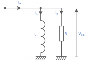
Figure 3 – Case 1 – Resister and Inductor in Parallel

The currents in the resistor and inductor are calculated in the time-domain from first principles.

$I_{R}\left ( t \right )=\frac{V_{out\left ( t \right )}}{R}\hspace{1.8cm} \text{The Fourier Transfer is:}\hspace{1.0cm} \hat{I_{R}}\left ( \omega \right )=\frac{\hat{V_{out}}\left ( \omega \right )}{R}$

$V_{out}\left ( t \right )=L\frac{dI_{L}\left ( t \right )}{dt}\hspace{1.0cm} \text{The Fourier Transfer is:}\hspace{1.0cm} \hat{V_{out}}\left ( \omega \right )=j\omega L\hat{I_{L}}\left ( \omega \right )$

An assumption is made that any initial currents are zero. Adding the currents:

$\hat{I_{in}}\left ( \omega \right )=\hat{I_{R}}\left ( \omega \right )+\hat{I_{L}}\left ( \omega \right )$

So, substituting:

$\hat{I}_{in}\left ( \omega \right )=\frac{\hat{V}_{out}\left ( \omega \right )}{R}+\frac{\hat{V}_{out}\left ( \omega \right )}{j\omega L}$

Rearranging:

$\hat{V}_{out}\left ( \omega \right )=\dfrac{\hat{I}_{in}\left ( \omega \right )}{\dfrac{1}{R}+\dfrac{1}{j\omega L}}$

The driving signal is a Dirac or impulse Function.

$I_{in}\left ( t \right )=\delta \left ( t \right )$

This excites all frequencies simultaneously and generates the ‘transfer function’ or the ‘frequency response’ of the circuit. The Fourier transform of the impulse function is: 1 (transfer pair 1), hence, the equivalent frequency-domain response is:

$\hat{V}_{out}\left ( \omega \right )=\dfrac{1}{\dfrac{1}{R}+\dfrac{1}{j\omega L}}$

Rearranging the transfer function to fit the standard form in the table:

$\hat{V}_{out}\left ( \omega \right )=j\omega R\left (\dfrac{1}{\dfrac{R}{L}+j\omega } \right )\hspace{3.4cm} \text{Equation 3}$

This is in standard form for converting back into the time-domain using transfer pairs 2 and 4 in the Fourier table:

$\text{Using}\hspace{0.7cm}e^{-\alpha t}u\left ( t \right )\Leftrightarrow \frac{1}{\alpha +j\omega }\hspace{0.7cm} \text{with}\hspace{1.0cm}\alpha =\frac{R}{L}\hspace{0.7cm} \text{and}\hspace{0.7cm}\frac{df\left ( t \right )}{dt}\Leftrightarrow j\omega F\left ( \omega \right )$

Then, in the time-domain:

$V_{out}\left ( t \right )=R\dfrac{d}{dt}\left ( e^{-\frac{Rt}{L}} \right )$

Giving

$V_{out}\left ( t \right )=-\frac{R^{2}}{L}e^{-\frac{Rt}{L}}\hspace{3.4cm} \text{Equation 4}$

Although equation 4 is correct, it is only correct for positive time. It is necessary to be more precise with the description. The following assumption must apply.

$V_{out}\left ( t \right )= \begin{cases} & -\frac{R^{2}}{L}e^{-\frac{Rt}{L}}\hspace{1.0cm}\text{ if } t \geq 0 \\ & 0\hspace{2.42cm}\text{ if } t < 0 \end{cases}\hspace{3.0cm} \text{Equation 5}$

A far more interesting way of developing equation 3 is to separate the expression into real and imaginary components. In effect, this turns the parallel connection into a series circuit. Multiply the top and bottom of equation 3 by the conjugate of the denominator:

$\hat{V}_{out}\left ( \omega \right )=\left (\dfrac{j\omega R}{\dfrac{R}{L}+j\omega} \right )\left ( \frac{\dfrac{R}{L}-j\omega}{\dfrac{R}{L}-j\omega} \right )$

Multiply this out to give:

$\hat{V}_{out}\left ( \omega \right )=-\left ( j\omega \right )^{2}\left ( \dfrac{R}{\dfrac{R^{2}}{L^{2}}+\omega ^{2}} \right )+j\omega\left ( \dfrac{\dfrac{R^{2}}{L}}{\dfrac{R^{2}}{L^{2}}+\omega ^{2}} \right )$

Putting this in standard form for transform pair 5 below:

$e^{-\alpha \left |t \right |}\Leftrightarrow \dfrac{2\alpha }{\alpha^{2} +\omega^{2} }\hspace{0.7cm} \text{with}\hspace{1.0cm}\alpha =\frac{R}{L}\hspace{0.7cm}$

$\hat{V}_{out}\left ( \omega \right )=-\left ( j\omega \right )^{2}\frac{L}{2}\left ( \dfrac{2\dfrac{R}{L}}{\dfrac{R^{2}}{L^{2}}+\omega ^{2}} \right )+j\omega \frac{R}{2}\left ( \dfrac{2\dfrac{R}{L}}{\dfrac{R^{2}}{L^{2}}+\omega ^{2}} \right )\hspace{3.0cm} \text{Equation 6}$

This is in the form:

$\hat{V}_{out}\left ( \omega \right )=R\left ( \omega \right )+jX\left ( \omega \right )$

where $R\left ( \omega \right )$ represents the resistive frequency response and $jX\left ( \omega \right )$ the reactive frequency response.

Equation 6 is in two parts, both in the frequency-domain. The real part is an even function whereas the complex part is an odd function. Using transform pair 5 and transform pair 2 in the Fourier transform table, the time-domain inverse can be written down:

Transforming equation 6 into the time-domain:

$V_{out}\left ( t \right )=-\frac{L}{2}\frac{d^2}{dt^2}\left ( e^{-\dfrac{R\left | t \right |}{L}} \right )+\dfrac{R}{2}\frac{d}{dt}\left ( e^{-\dfrac{R\left | t \right |}{L}} \right )\hspace{3.0cm} \text{Equation 7}$

Transforming the $j\omega$ term in equation 6 gives rise to a time-domain derivative in equation 7. Similarly, the $\left ( j\omega \right )^{2}$ term gives rise to a second order derivative. The derivatives are a little tricky and involves the chain rule.

Due to the absolute operator $\left | t \right |$ , the derivatives are continuous everywhere except at t=0. The result is undefined at t=0. The following calculations illustrates one possible evaluation method.

Let:

$f\left ( t \right )=e^{\gamma \left | t \right |}\hspace{0.5cm} \text{and define}\hspace{0.5cm}\left | t \right |=\sqrt{t^{2}}\hspace{0.5cm}\text{so}\hspace{0.5cm}f\left ( t \right )=e^{\gamma \left ( t^{2} \right )^{\frac{1}{2}}}$

Using the chain rule, the first derivative is:

$f'\left ( t \right )=e^{\gamma \left ( t^{2} \right )^{\frac{1}{2}}}\gamma \frac{1}{2}\left ( t^{2} \right )^{-\frac{1}{2}}2t$

Tidy up:

$f'\left ( t \right )=\gamma e^{\gamma \left ( t^{2} \right )^{\frac{1}{2}}}\left ( t^{2} \right )^{-\frac{1}{2}}t\hspace{3.0cm} \text{Equation 8}$

Hence the first derivative can be expressed as:

$f'\left ( t \right )=\gamma e^{\gamma \left ( t^{2} \right )^{\frac{1}{2}}}\frac{t}{\left | t^{2} \right |}$

$f'\left ( t \right )=\gamma e^{\gamma \left | t \right |}sgn\left ( t \right )\hspace{3.0cm} \text{Equation 9}$

Where:

$sgn\left ( t \right )=\frac{t}{\sqrt{t^{2}}}$

and

$sgn\left ( t \right )=\begin{cases} &1\hspace{1.0cm} \text{ if } t > 0 \\ &0\hspace{1.0cm} \text{ if } t = 0\\ &-1\hspace{0.66cm} \text{ if } t <0 \end{cases}$

The second derivative is found by differentiating equation 8. This is a product of three ‘t’ terms. Using the product rule and the chain rule, the solution can be written down in one go.

differentiating: $\gamma e^{\gamma \left ( t^{2} \right )^{\frac{1}{2}}}\left ( t^{2} \right )^{-\frac{1}{2}}t$

Gives:

$f{}''\left ( t \right )=\gamma e^{\gamma \left ( t^{2} \right )^{\frac{1}{2}}}\left [ t\left ( -\frac{1}{2}\left ( t^{2} \right )^{-\frac{3}{2}} \right )2t +1\left ( t^{2} \right )^{-\frac{1}{2}} \right ]+\gamma ^{2}e^{\gamma \sqrt{t^{2}}}\frac{t}{\sqrt{t^{2}}}\frac{t}{\sqrt{t^{2}}}$

Tidy up:

$f{}''\left ( t \right )=\gamma e^{\gamma \left ( t^{2} \right )^{\frac{1}{2}}}\left [ -\frac{t^{2}}{\left ( \sqrt{t^{2}} \right )^{3}} +\frac{1}{\sqrt{t^{2}}}\right ]+\gamma ^{2}e^{\gamma \sqrt{t^{2}}}sgn^{2}\left ( t \right )$

Here:

$sgn\left ( t \right )=\frac{t}{\sqrt{t^{2}}}=\frac{t}{\left | t \right |}$

Another tidy up:

$f{}''\left ( t \right )=\gamma e^{\gamma \left ( t^{2} \right )^{\frac{1}{2}}}\left [ -\frac{t^{2}}{\left ( \sqrt{t^{2}} \right )^{3}} +\frac{t^{2}}{\left ( \sqrt{t^{2}} \right )^{3}}\right ]+\gamma ^{2}e^{\gamma \sqrt{t^{2}}}sgn^{2}\left ( t \right )$

The first term is zero. Also, $sgn^{2}\left ( t \right )=1$ (t>0, t<0). The derivative is not defined for t=0.

The second derivative is:

$f{}''\left ( t \right )=\gamma ^{2}e^{\gamma \left | t \right |}\hspace{3.0cm} \text{Equation 10}$

Now substitute equations 9 and 10 into equation 7 with $\gamma =-\frac{R}{L}$
Restating equation 7:

$V_{out}\left ( t \right )=-\frac{L}{2}\frac{R^{2}}{L^{2}}e^{-\dfrac{R\left | t \right |}{L}} -\dfrac{R}{2}\frac{R}{L} e^{-\dfrac{R\left | t \right |}{L}}sgn\left ( t \right )$

Giving the final solution:

$V_{out}\left ( t \right )=-\frac{R^{2}}{2L}e^{-\dfrac{R\left | t \right |}{L}} -\frac{R^{2}}{2L} e^{-\dfrac{R\left | t \right |}{L}}sgn\left ( t \right )\hspace{3.0cm} \text{Equation 11}$

As expected, the even real part of equation 6 is transformed under the Fourier transform from the frequency-domain into an even function R(t) in the time-domain symmetrical about t=0. Similarly, the complex part of equation 6 is transformed into an odd function X(t). This solution is defined for all time apart from t=0. Note: for t > 0, equation 11 is exactly the same as equation 4.

Plotting equation 11 is interesting. For this plot R=20 Ω and L=1 H

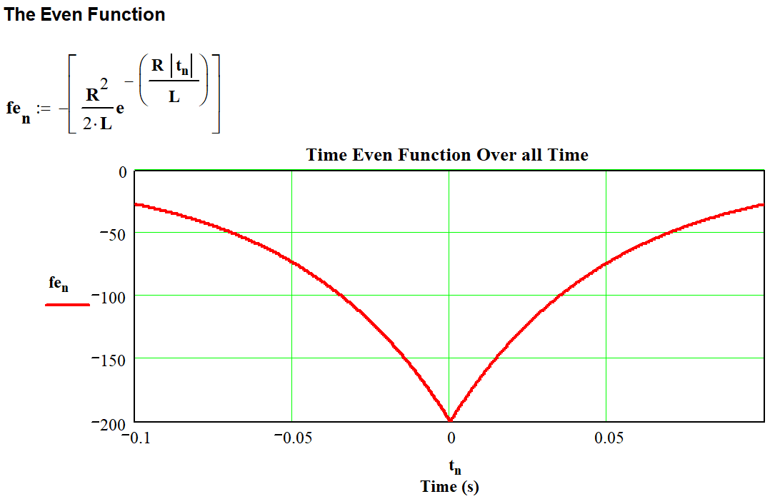
Figure 4 – Resistor Inductor Even Plot over all Time

Figure 4 shows a plot of the even function which is symmetrical around t=0. For the components shown, the maximum value at t=0 works out at:

$-\frac{R^{2}}{2L}=-200$

The plot, figure 5, shows the odd function. The signum(t) (in the plots) is the same as the sgn(t) function.

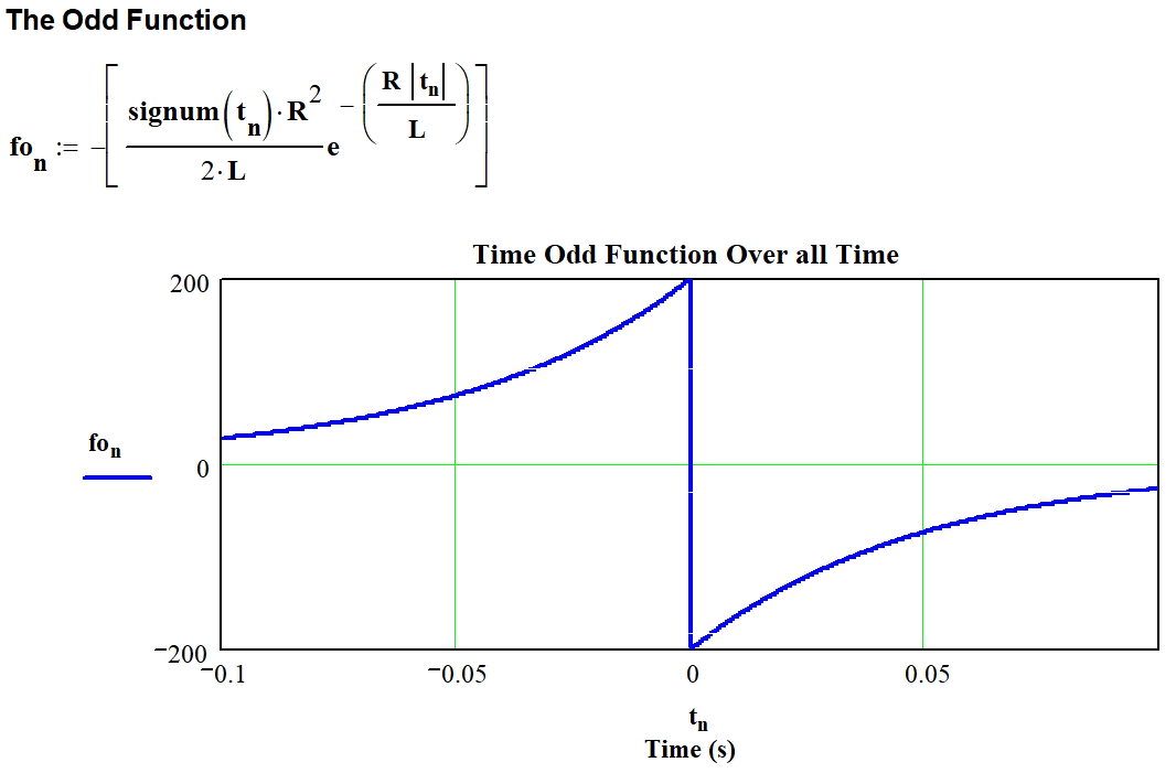
Figure 5 – Resistor Inductor Odd Plot over all Time

Adding the even and odd time-domain functions (As described in equation 11), the time-domain function of the RC network is revealed over all time.

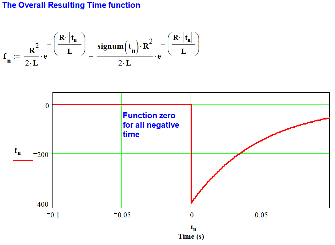
Figure 6 – The Combined Even and Odd function Together Produces f(t)

Figure 6 illustrates that the function is zero for all negative time. The response is identical to that described by equation 5. However, the calculation required no assumptions to reach this conclusion.

The relationship between Real and Imaginary Parts of Equation 3

Repeating Equation 11:

$V_{out}\left ( t \right )=-\frac{R^{2}}{2L}e^{-\dfrac{R\left | t \right |}{L}} -\frac{R^{2}}{2L} e^{-\dfrac{R\left | t \right |}{L}}sgn\left ( t \right )\hspace{3.0cm} \text{Equation 11}$

This is in the form:

$V_{out}\left ( t \right )=f_{Even}\left ( t \right )+f_{Odd}\left ( t \right )$

For the time-domain function to add to exactly zero for all negative time then:

$f_{Odd}\left ( t \right )=f_{Even}\left ( t \right )\hspace{1.1cm} \text{t}> 0$

$f_{Even}\left ( t \right )=-f_{Odd}\left ( t \right )\hspace{0.8cm} \text{t}< 0$

This implies:

$f_{Odd}\left ( t \right )=f_{Even}\left ( t \right )sgn\left ( t \right )\hspace{4.1cm} \text{Equation 12}$

$f_{Even}\left ( t \right )=f_{Odd}\left ( t \right )sgn\left ( t \right )\hspace{4.1cm} \text{Equation 13}$

Equations 12 and 13 are products in the time domain. These can be transformed into convolutions in the frequency domain using the frequency convolution theory.

$f_{1}\left ( t \right ).f_{2}\left ( t \right )\Leftrightarrow \frac{1}{2\pi }\int_{-\infty }^{\infty }F_{1}\left ( y \right )F_{2}\left(\omega -y \right )dy$

Other terms transform into the frequency domain as:

$f_{Odd}\left ( t \right )\Leftrightarrow jX\left ( \omega \right )$

$f_{Even}\left ( t \right )\Leftrightarrow R\left ( \omega \right )$

and

$sgn\left ( t \right )\Leftrightarrow \frac{2}{j\omega }\hspace{3.0cm} \text{Transfer Pair 6 on the Table}$

Hence from equation 12:

$jX\left ( \omega \right )=\frac{1}{2\pi }\frac{2}{j}\int_{-\infty }^{\infty}\frac{1}{\omega -y}R\left ( y \right )dy$

And, from equation 13:

$R\left ( \omega \right )=\frac{1}{2\pi }\frac{2}{j}\int_{-\infty }^{\infty}\frac{1}{\omega -y}jX\left ( y \right )dy$

Cancelling the ‘j’ terms and tidying up, the two Hilbert Transform Pairs emerge:

Hilbert Transform Pair

$X\left ( \omega \right )=-\frac{1}{\pi }\int_{-\infty }^{\infty }\frac{R\left ( \omega \right )}{\omega -y}dy\hspace{3.0cm} \text{Equation 1}$

$R\left ( \omega \right )=\frac{1}{\pi }\int_{-\infty }^{\infty }\frac{X\left ( \omega \right )}{\omega -y}dy\hspace{3.4cm} \text{Equation 2}$

Hence, equations 1 and 2 must hold if the circuit is causal (which it is because it exists in the real world). It means that any inductor must have a frequency dependent resistive component that complements the inductive response. All inductors must be lossy.

Sorry for the tedium.

73 Chris