Introduction
In theory, topband is an easy band to get on. A length of wire will tune if it is reasonably long and fed against earth using a tuner. However, it is very difficult to make an efficient antenna. By efficient, I mean 30% or more. It is even more difficult to build efficient antenna if you are limited by small gardens and irritating neighbours.
This document records the results from a number of experiments performed at my suburban QTH. Restrictions include a pole on the side of the house at a height 36 ft and a tree/pole 105 ft down the garden approximately 35 ft high. Every QTH is different of course with a different set of limitations. However, many of the conclusions that emerged from this work should apply to other scenarios.
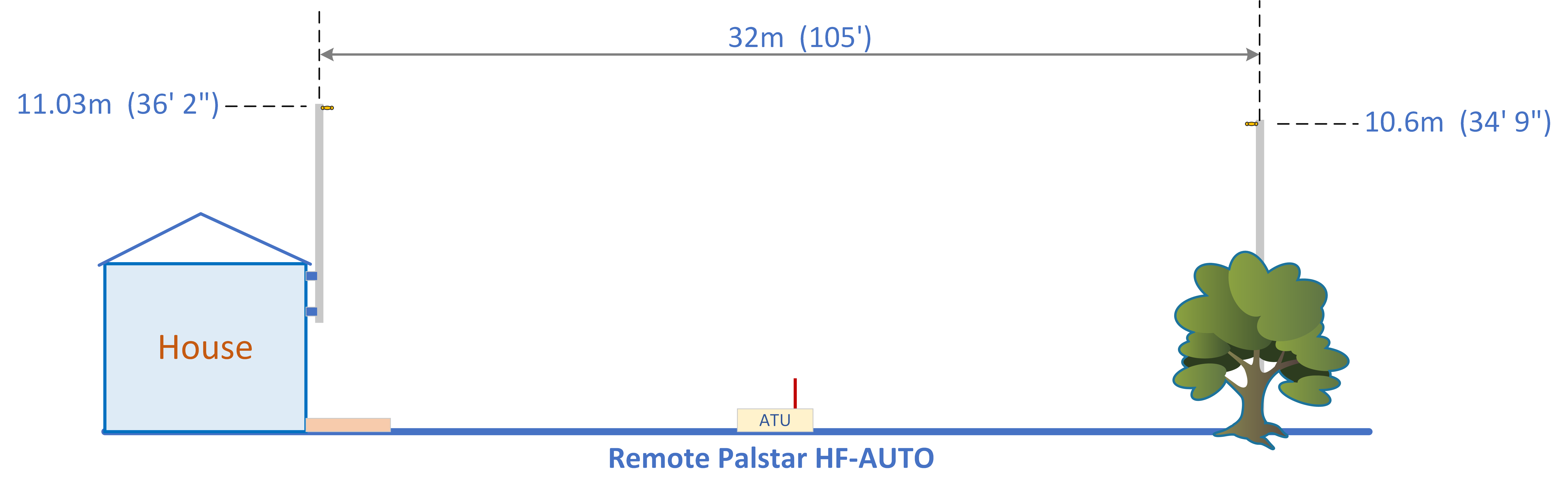
Figure 1 – The limiting Constraints at G4AKE QTH
Most of the antenna tried were end-fed and required an earth system. The feed point consisted of a Palstar HF-Auto tuning unit housed inside an outbuilding positioned midway along the garden. For this reason, the earth radials radiated from that point into the extremities of the garden. Figure 2 shows a scaled plan view of the complete radial system consisting of 18 bare copper wires buried approximately 10 cm beneath the soil. The wire diameter was 1.5 mm.
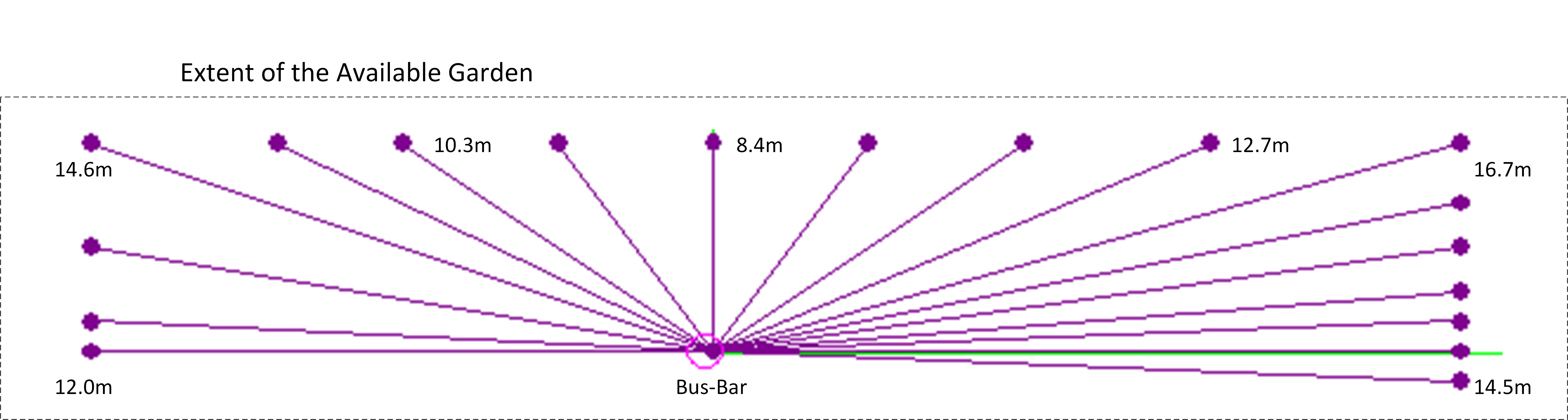
Figure 2 – Plan View of the G4AKE Earth Radial System
Additional earth rods driven into the ground near the feed point made no perceivable difference to the feed impedance or radiated signal. A local WEB SDR receiver proved a useful tool for comparing the radiated signals.
The radial system is far from optimal but it did represent a considerable physical effort. Many gardens have inaccessible areas such as garages, patios and ponds. Sometimes even a modest earth system is difficult to realise. The longest radial is only 16.7 m (55 ft) in length and the shortest is 8.4 m (27 ft). The text books suggests that we should aim for 120 radials of length 132 ft or more radiating equally around the feed point – dream on!
I wanted to quantify these experiments using practical methods but this turned out impractical. Local propagation is not that helpful in determining efficiency or low angle propagation of the antenna. I concluded that the best methodology is to model different antenna under the same restrictions and see how they perform. The modelling software NEC2 is capable of impressive results if the rules are followed.
The key to good modelling is to check the model against reality. A good check is to calculate the complex antenna feed impedance at points in the band and compare them against measured values to see if the magnitudes and behaviours are similar. Even if absolute values diverge from reality, the comparisons remain useful.
4NEC2
I use 4NEC2 (v 5.8.16) which is excellent in my opinion. It can be difficult if you are starting from scratch with no knowledge of the software or of NEC2. 4NEC2 implements the Arnold Sommerfeld integral solution for wires near to the earth and allows the user to select standard ground conditions described in the software as ‘poor’, ‘moderate’, ‘average’, ‘good’ and ‘dry’. I found that the ‘Average’ ground condition (Dielectric constant =13 and conductivity = 0.005 S) provided the best fit for me. You would have to experiment to find the best fit for the earth at your QTH.
NEC2 cannot model radials underground so I use a technique of laying a virtual radial system 0.1 m above the air/ground interface. According to “ITU Handbook on Ground Wave Propagation”, the skin depth of the ground at 1.93 MHz is approximately 5 m so the RF interface between air and ground is not well defined in any case. This method seemed to work well. As an example, modelling a strapped G5RV against ground with radials raised at different heights above ground gave the following efficiencies: 0.01 m 16.31%, 0.1 m 19.3%, 0.2 m 19.71% and 0.3 m 20.28%.
I decided to use 0.1 m as the lowest stable figure but I accept that the efficiencies calculated may be optimistic. The important part is to apply the same conditions to all the antenna on test. This ‘test’ provided an immediate conclusion: Raised radials are probably more efficient than buried systems.
Test Conditions
– The antenna wire loss resistance is not included in these calculations.
– Antenna support 1 at the house: 11.03 m high (See Figure 1).
– Antenna support 2 down the garden: 10.66 m high (See Figure 1).
– Height at the centre for the G5RV: 8 m.
– Earth: Standard G4AKE radials (18 Radials) – See Figure 2.
– Earth type: Average (Dielectric constant =13 and conductivity = 0.005 S).
– Test frequency: 1.930 MHz.
– The day time ground/surface wave is calculated at 143 km in μV/m. Using this this distance enables me to compare results on a WEB-SDR receiver at a distance of 143 km from my QTH. I cannot vouch for the calibration of the WEB-SDR and the antenna correction factor used to convert from V/m to V. However, it is a useful comparison and provides a ball-park indication of validity. Ground wave is calculated and measured for 10 W output power. The practical measurements were made at midday to ensure ground wave conditions.
Please note: I sometimes present results to three decimal places or more which is ridiculous. I make less mistakes using the clip-board. So please forgive me.
Antenna Configurations Tested
(1) Vertical 18.7 m or 61 ft high with centre loading coil at a height of 9.6 m (100 uH).
(2) 100 ft unloaded vertical (Impractical at my QTH but interesting).
(3) 132 ft vertical, full size no loading (Impractical at my QTH but interesting).
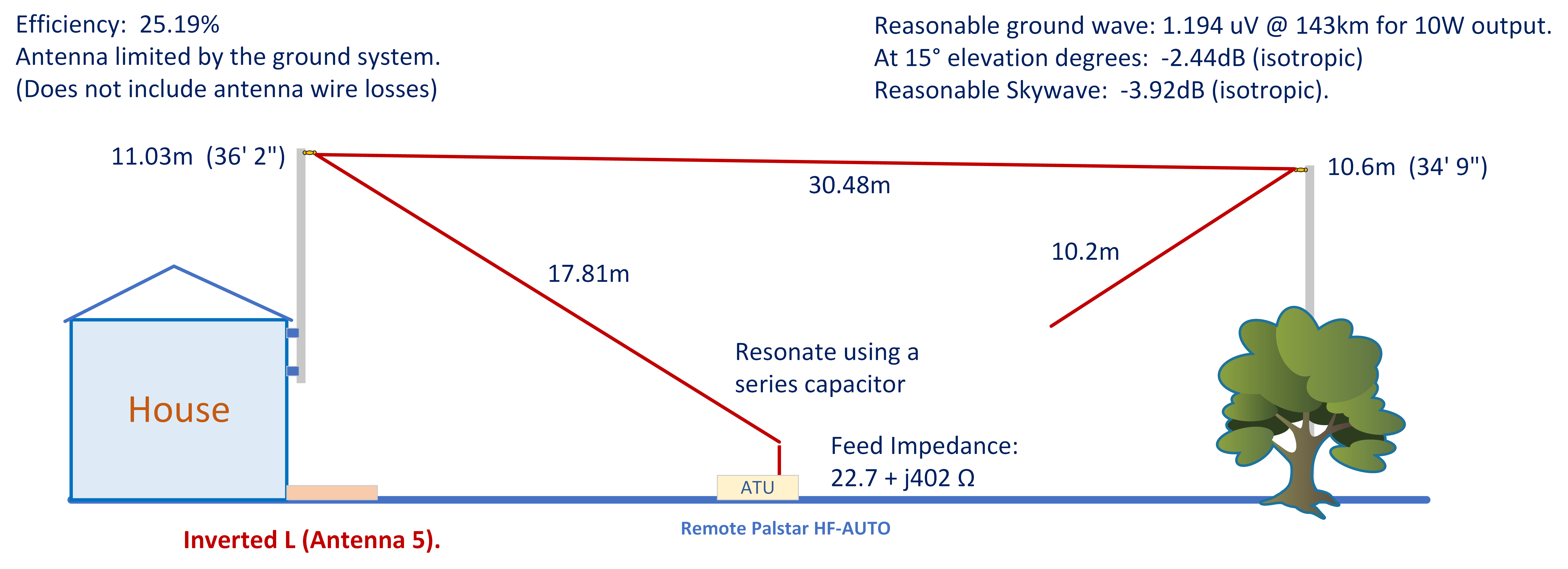
(4) Inverted L top 30.48 m, feed wire 17.81 m feed point 1.8 m high.
(5) Inverted L top 30.48 m, feed wire 17.81 m, tail loading of 10.2 m drooping towards feed point.
(6) Inverted L top 30.48 m, feed wire 17.81 m, tail loading of 17.5 m drooping towards feed point.
(7) Delta loop made up of the same elements in (6).
(8) The Delta loop in (7) powered in common mode.
(9) Horizontal halfwave dipole above the earth mat. The height is 60 ft – Impractical at my QTH.
(10) As (9) but no G4AKE earth mat.
(11) Horizontal halfwave dipole above the earth mat. Height is 38 ft (Impractical at my QTH).
(12) Halfwave is at 38 ft. No G4AKE earth mat.
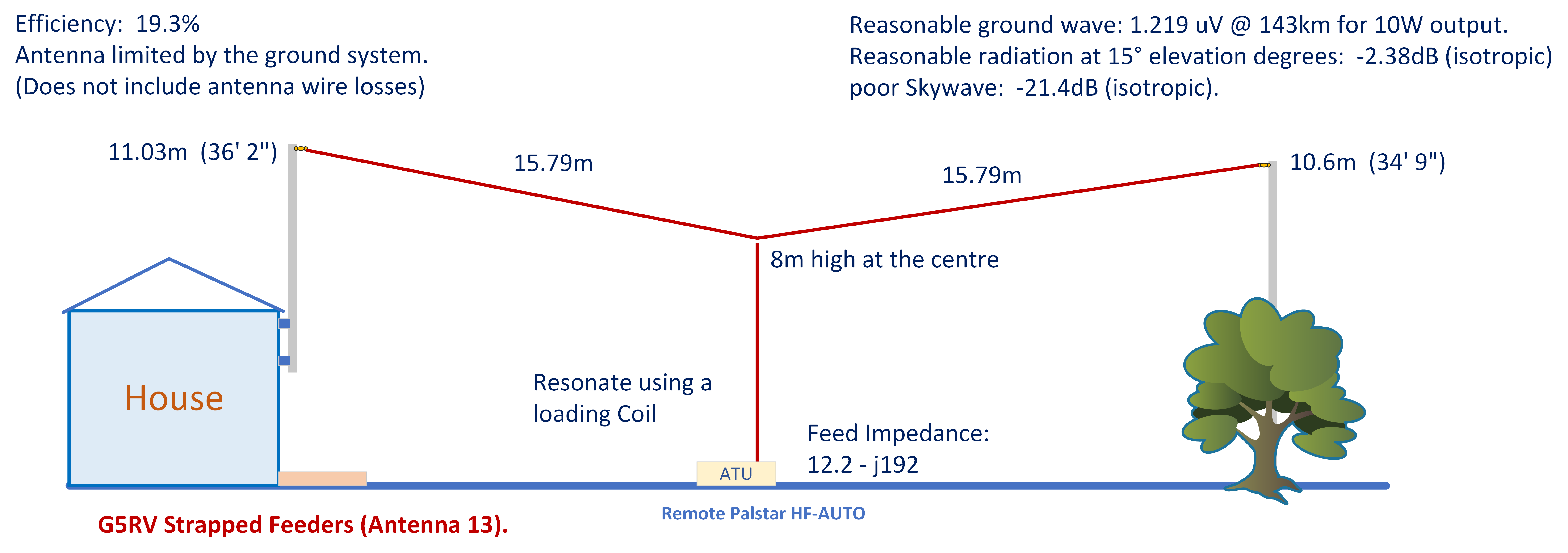
(13) A G5RV type dipole with 102 ft top fed by strapped feeders. Feeder length: 8 m.
(14) The G5RV type dipole in (13) is extended on each end of the dipole by wires 5 m long.
The following table provides a summary of the results. Note that the Field Strength estimates at 15° and vertical incidence are expressed as dB relative to an isotropic source. Hence, a figure of -3 dB is better than -6 dB. An isotropic source is one that radiates in all directions equally.
| Description | Note | Tried and Tested | Impedance (Ω) | Efficiency (%) | Ground Wave @143km (10W) | Field (NVIS) Straight Up | Field at 15° Elevation (Max) |
|---|---|---|---|---|---|---|---|
| Vert 61 ft (1) | Ideal 100 uH loading coil | Yes | 23.5 + j16.1 | 25.08 | 1.384 μV/m | -25 dB | -1.35 dB |
| Vert 100 ft (2) | No Loading Coil | No | 30.2 - j204 | 28.24 | 1.494 μV/m | -25.7 dB | -0.73 dB |
| Vert 132 (3) | No loading coil | No | 57 + j27.4 | 30.76 | 1.593 μV/m | -28.8 dB | -0.25 dB |
| Inverted L (4) | Two wires | Yes | 19.5 + j159 | 20.8 | 1.196 μV/m | -10.5 dB | -2.53 dB |
| Inverted L (5) | Three wires | Yes | 22.7 + j402 | 25.19 | 1.194 μV/m | -3.92 dB | -2.44 dB |
| Inverted L (6) | Extended further | Yes | 27.4 + j819 | 32.95 | 1.195 μV/m | 0.64 dB | -2.26 dB |
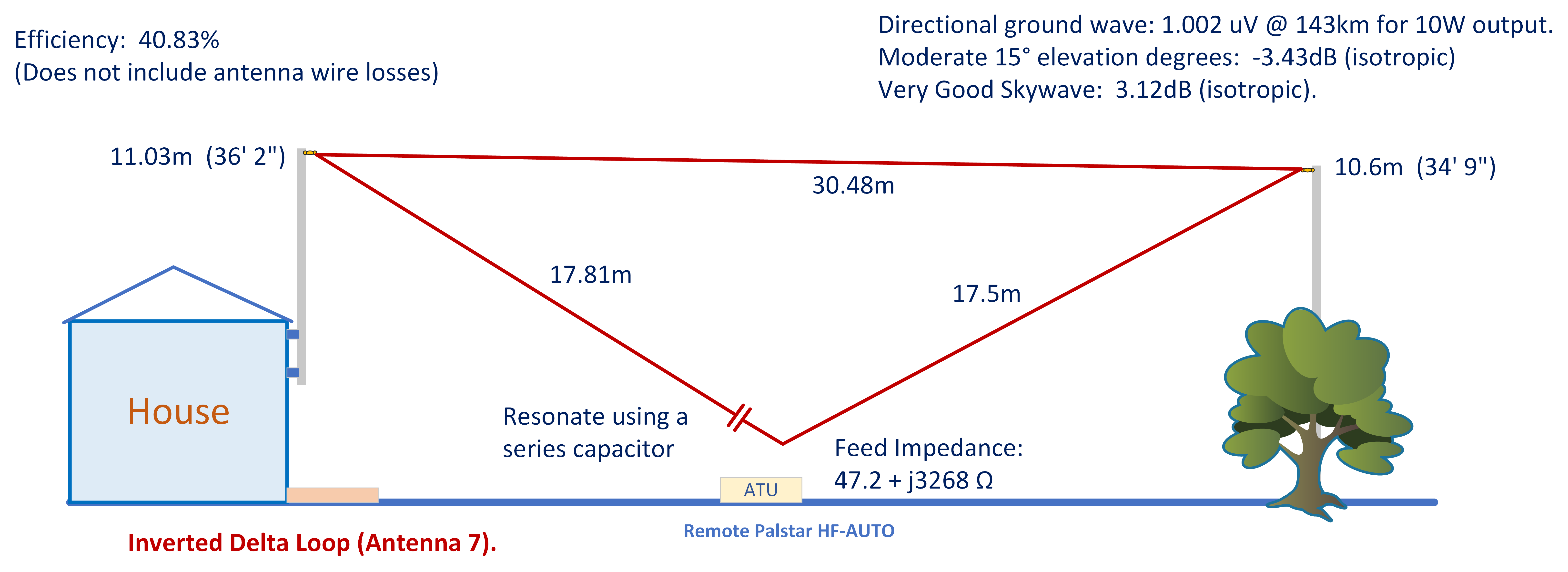
| Delta Loop (7) * | Inverted | Failed | 47.2 + j3268* | 40.83 | 1.002 μV/m | 3.12 dB | -3.43 dB |
| Delta Loop (8) | Delta in CM | Yes | 12.4 - j90.8 | 19.14 | 1.214 μV/m | -21.4 dB | -2.44 dB |
| Halfwave dipole (9) | Height at 60 ft | No | 47.1 + j3.95 | 63.43 | 0.337 μV/m | 6.35 dB | -3.71 dB |
| Halfwave dipole (10) | As (9) No Earth Mat | No | 46.3 + j4.95 | 65.05 | 0.376 μV/m | 6.46 dB | -3.61 dB |
| Halfwave dipole (11) | Height at 38 ft | No | 39.18 + j4.59 | 39.18 | 0.417 μV/m | 4.3 dB | -6.29 dB |
| Halfwave dipole (12) | 38 ft no earth mat | No | 37.3 - j3.12 | 41.95 | 0.419 μV/m | 4.6 dB | -5.00 dB |
| G5RV (13) | Standard 8m centre | Yes | 12.2 - j192 | 19.3 | 1.219 μV/m | -21.4 dB | -2.38 dB |
| G5RV Extended (14) | Tails 5m each side | Yes | 12.9 - j119 | 18.93 | 1.202 μV/m | -22.5 dB | -2.49 dB |
* I Failed to get the inverted Delta Loop (7) to work with the dimensions shown
The third table column indicates the antennas tried and tested. In these cases, the practical antennas were checked against the NEC2 model for validity. For example, the calculated G5RV (13) showed an efficiency of 19.3% and resistive feed impedance of 12.2 Ω. When measured at resonance with a real loading coil, the measured resistance was 13.0 Ω. Incidentally, without any effort, it was very easy to add several ohms to the feed impedance just by using a roller-coaster inductor rather than using my large 20 cm diameter 8 mm tubular coil! Beware!
61 ft Vertical (Antenna 1) – Tried and Tested
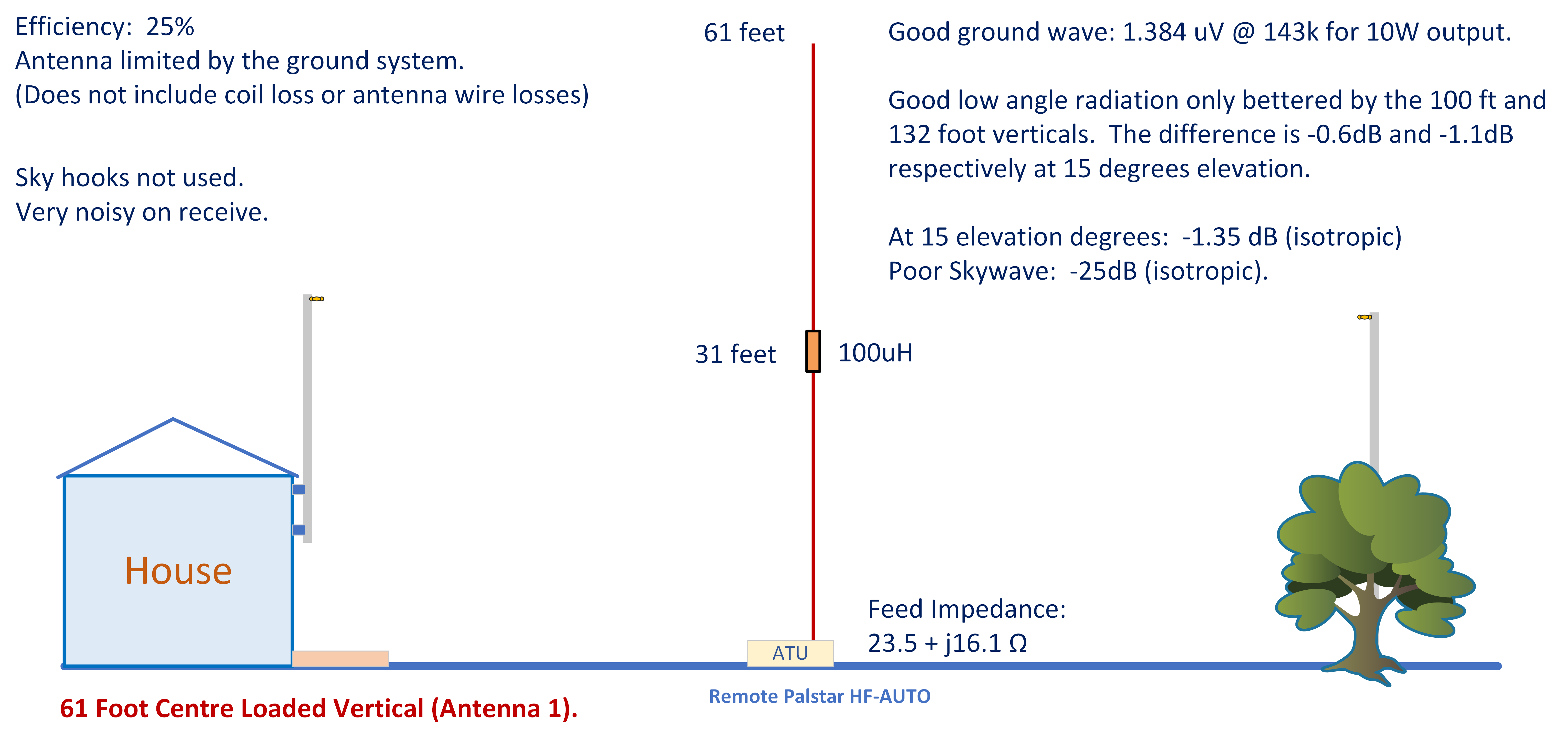
The vertical section consisted of aluminium tube of height 31 ft pivoted at the base. The remainder comprised a fibreglass fishing roach pole with copper wire taped to the outside. I avoided the urge to wind the wire into a helix as this just makes the simulation difficult.
The loading coil employed 8 mm diameter copper tubing wound on to a 20 cm diameter former (This was a plastic paint container). The coil was heavy and self-supporting. The bottom end of the coil bolted directly to the alloy tube. The top end was attached to the fibre glass rod using adhesive tape. The whole antenna could be erected and lower by one person although it did involve some effort.
This was a great antenna for local ground wave nattering and it seem to work quite well with DX. However, it was hopeless for ‘inter G’ working where NVIS, or Near Vertical Incidence Skywave propagation is desirable. In fact, the predicted vertical propagation is down 25 dB on an isotropic source. I doubt very much that I achieved 25% efficient with the practical antenna. Additional losses in the wires and the loading coil probably reduced the overall efficiency to around 15 – 20% or possibly lower.
23.5 Ω is difficult to load without an ATU. Balan transformers can easily provide 4:1 impedance transformation but 2:1 is more difficult. The remote ATU, despite its size, introduced significant losses when used to match low impedance loads.
100 foot Vertical (Antenna 2) – Fantasy Antenna
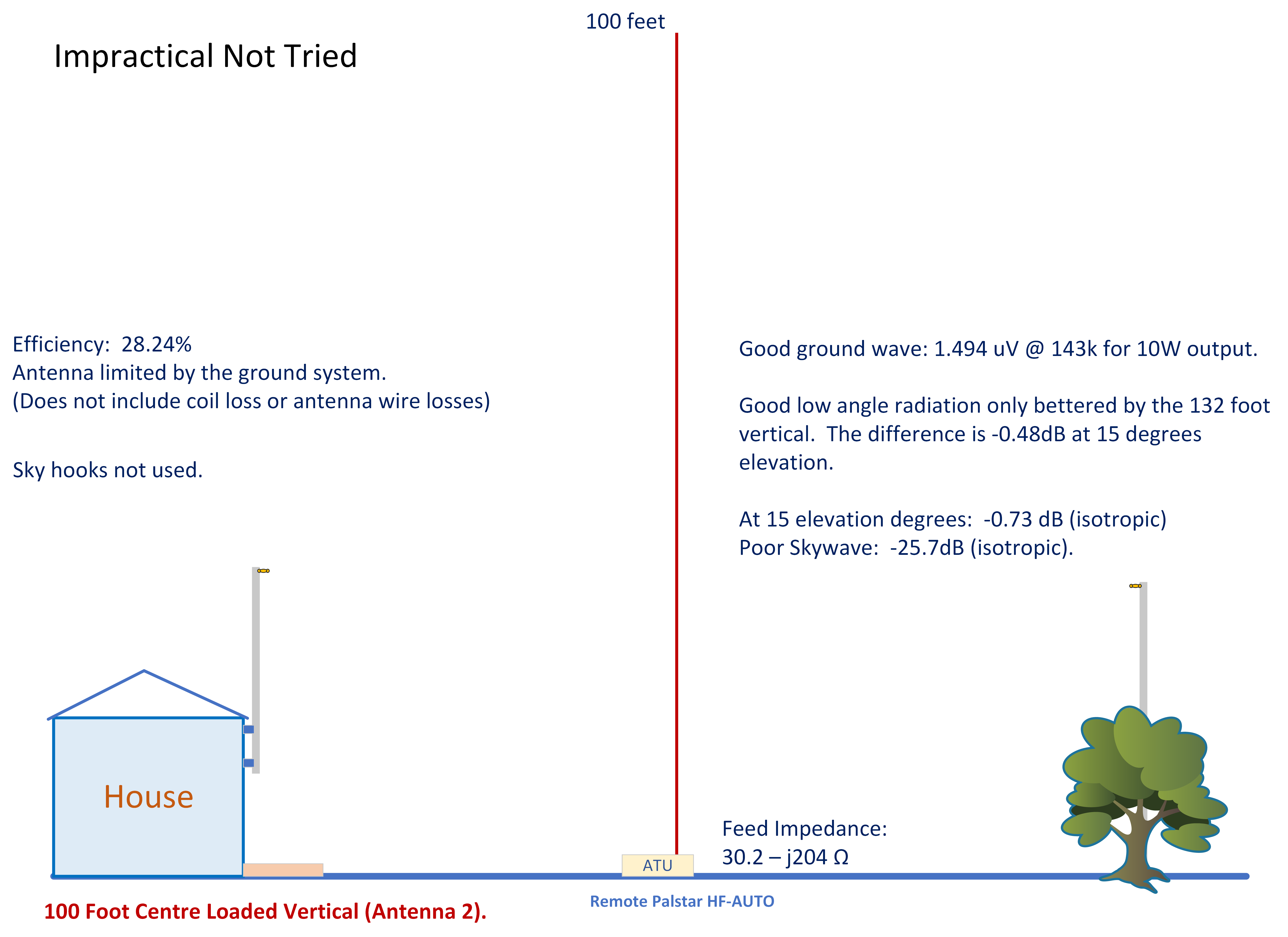
I did not try this antenna. My neighbours would have a fit. Surprisingly, the predicted performance is only slightly better than the 61 ft vertical.
To be fair, the 100 ft antenna in this configuration must be bottom loaded whereas the 61 ft element is centre loaded. I suspect that the earth system is just too small for this height. It seems that an unwritten rule states: “the antenna height must not be greater than the radius of the radial mat”. In practice, if you go to the trouble of building a tall vertical, it is essential that you spend as much time on the radial system if you want to see any real benefit. Efficiency increased by only 3.16%
The ground wave signal at 143 km increased by only 0.66 dB compared with the 60 ft vertical. At 15° elevation, the increase is only 0.62 dB. It would be much easier to achieve this level of performance by improving the 61 ft vertical or just by running slightly more power!
132 ft Vertical (Antenna 3) – Fantasy Antenna
The 132 ft (40 m) vertical is a self-resonant antenna not requiring loading coils so is likely to be the most efficient vertical and best performer. It is totally impractical but interesting as a thought experiment.
Using the ‘G4AKE’ 18 radials and ‘Average’ ground setting, the efficiency is no better than 30.76%. It is not much better than the 25% efficiency of the 61 ft vertical – a huge disappointment – I really wanted one. As an indicator, if the earth is replaced by ‘Good’ (Dielectric constant =17 and conductivity = 0.015 S), then the efficiency jumps to 46% and the Field strength at 15° increased by approximately 1.95 dB and is then 1.7 dB above the isotropic source figure.
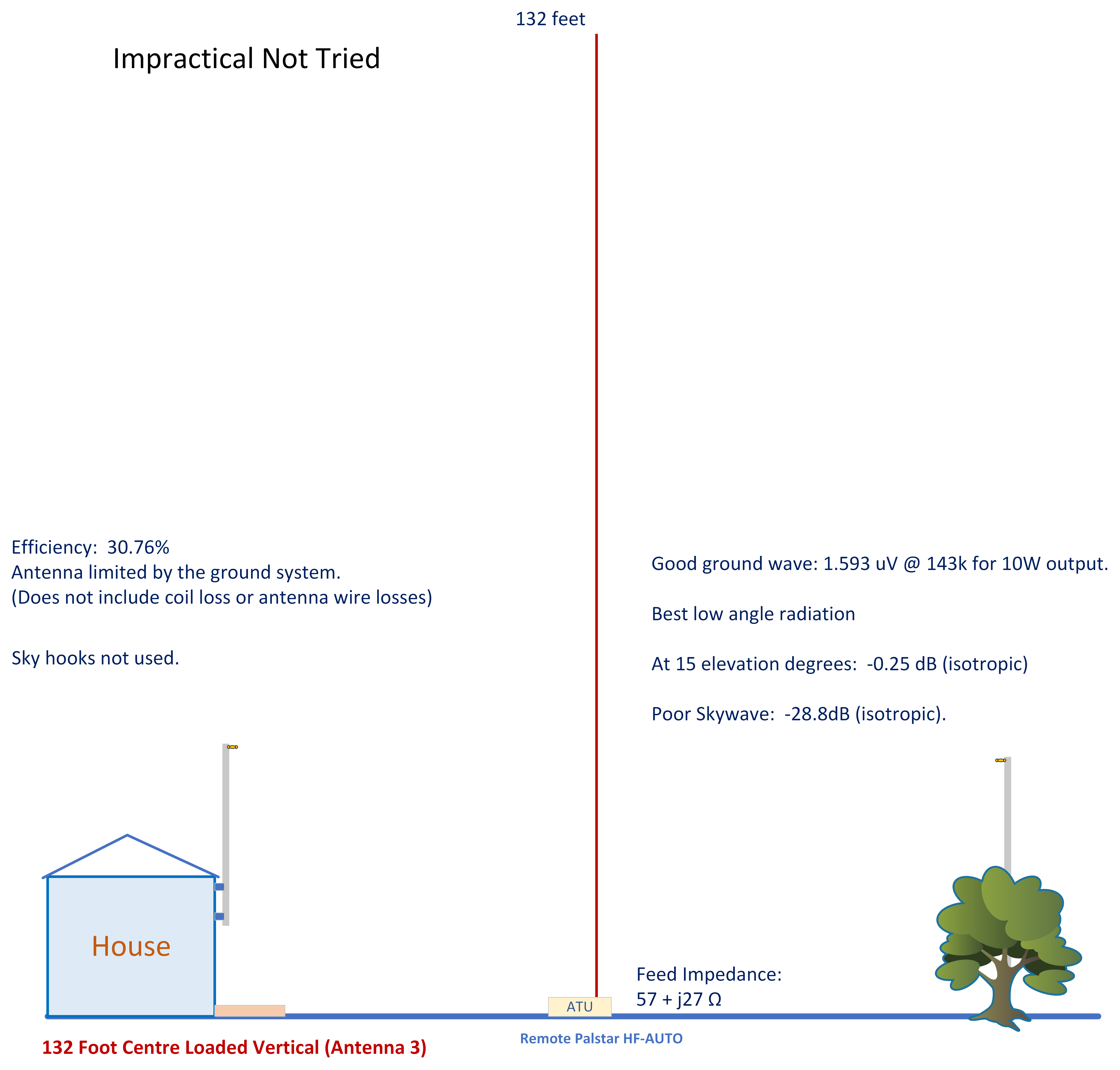
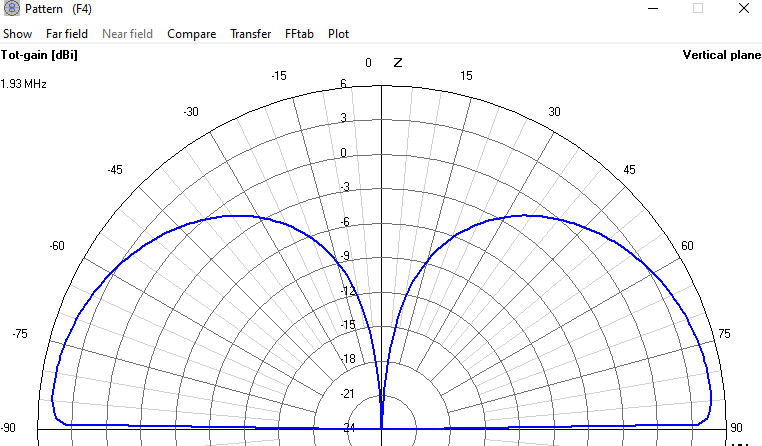
Figure 3 – Quarter Wave Vertical above G4AKE Radials and Sea Water
In case you are wondering, sea water takes the antenna efficiency up to 93.6%. Figure 3 shows the vertical radiation pattern of the Antenna over a sea water ground (still using the radial mat).
The amazing part is that the radiation maximises at angles close to the ground. The antenna generates maximum output at around 5° elevation. This would be superb for DX. This illustrates just how mediocre ground ruins the performance of a vertical.
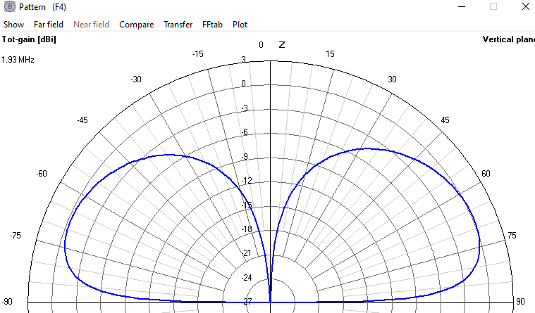
Figure 4 – Quarter Wave Vertical above G4AKE Radials and Average Ground
Even more remarkable is the ground wave. With ‘Average’ ground, the ground wave signal at 143 km is approximately 1.593 μV/m for 10 W. With seawater as the ground, this leaps up to around 200 μV/m, an increase of 40 dB! That is an enormous increase. In fact, I didn’t believe the result so I looked it up in ITU-R P.368. The chart closest to the test conditions suggested 177 μV/m at 143 km (That was for a dielectric constant = 81 and conductivity = 5 S rather than dielectric constant = 70 and conductivity = 5 S). I concluded that these results are probably correct. Note that the 40 dB increase would only apply if the whole 143 km path was over sea water!
Figure 4 shows the same ‘fantasy’ antenna (Quarter wave Vertical) over the same 18 radials and ‘Average’ soil. The radiation at 5° drops by 9.3 dB. The cancellation at low angles is due to phase reversal below the Brewster angle. This occurs due to the air and the dielectric interface.
Inverted L – Tried and Tested (Antenna 4)
The inverted L is very practical but only 20.8% efficient (ignoring wire losses). This antenna fits the garden very well and is physically resilient in the wind. However, the performance is mediocre. It is not the best antenna for ground wave or low angle radiation and relatively poor for skywave with NVIS (Near Vertical Incidence Skywave) propagation down 10.5 dB on an isotropic source.
The only good feature is the inductive feed reactance that means a series capacitor can be used to tune it. Capacitors exhibit less series loss resistance than inductors.
Tuning with a series capacitor will leave approximately 19.5 Ω to match. A 4:1 impedance balun will result in a VSWR of 1.56. Without the balun, the VSWR shoots up to 2.6 if you attempt to tune 19.5 Ω directly. Ideally, avoid a tuning unit.
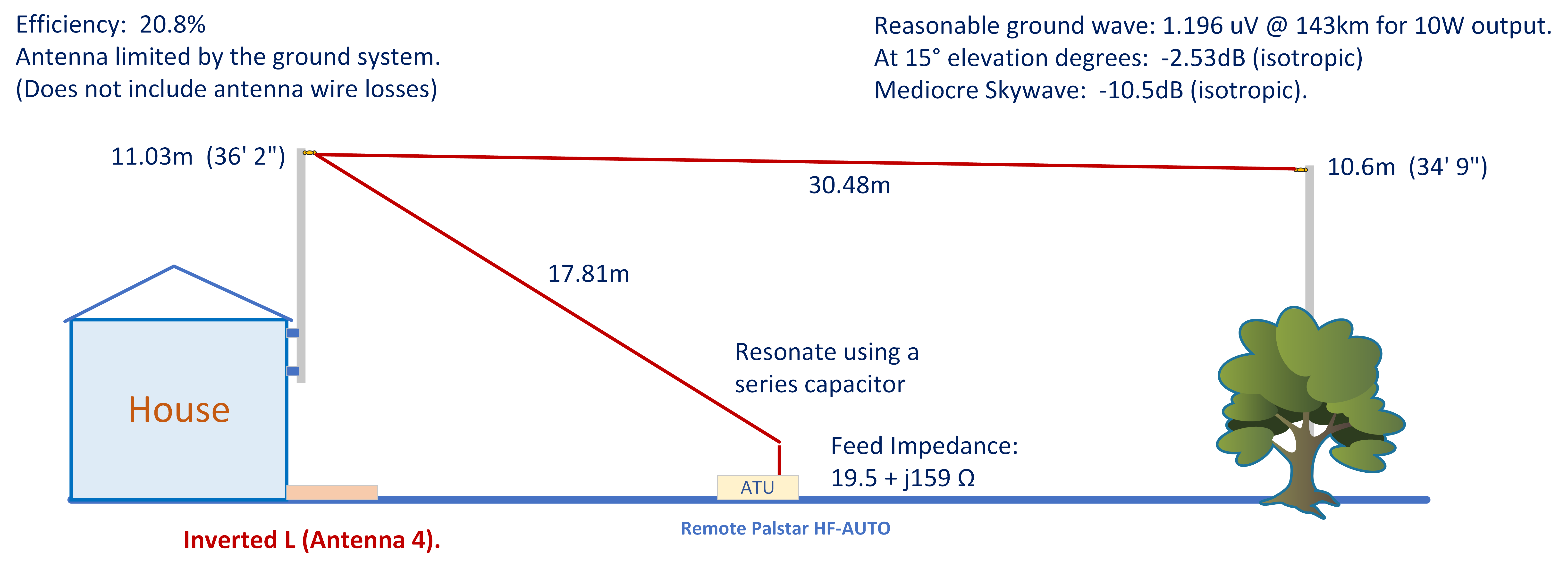
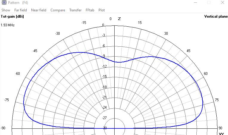
Figure 5 – Vertical Plane – Simple Inverted L
The horizontal pattern at 143 km remained largely unidirectional.
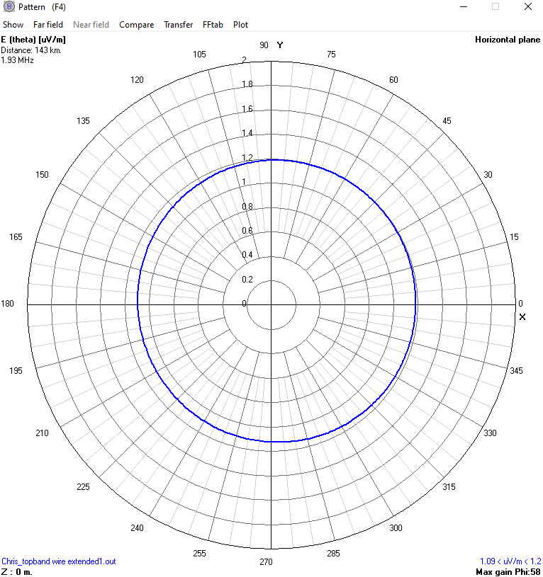
Figure 6 – Inverted L – Horizontal Surface Wave Pattern at 143km
Another disappointing feature is the lack of multiband operation. The Palstar HF-AUTO failed to find solutions on 80 m, 40 m and 10 m (The series capacitor for 160m not fitted).
Extended Inverted L (Antenna 5) – Tried and Tested
According to NEC2, adding 10.2 m of wire on the end of the inverted L increased the efficiency by almost 5%. The corresponding increase in the NVIS was 6.58 dB.
This version of the inverted L is much better for inter-G working and slightly better at low angles (15°) in some directions.
This antenna was used on 160 m in December 2019 on WSPR with 20 W over several nights. The best DX was BD7 at 9538 km with a report of -25 dB (Not exactly band crunching). Other stations in the USA approximately 5000 km to 6500 km away could also hear the signal. In this instance, I used a PALSTAR HF-Auto to match the antenna. This is not a bad all-round antenna. The disadvantage is the awkward feed impedance that forces the use of an ATU and the introduction of ATU related losses.
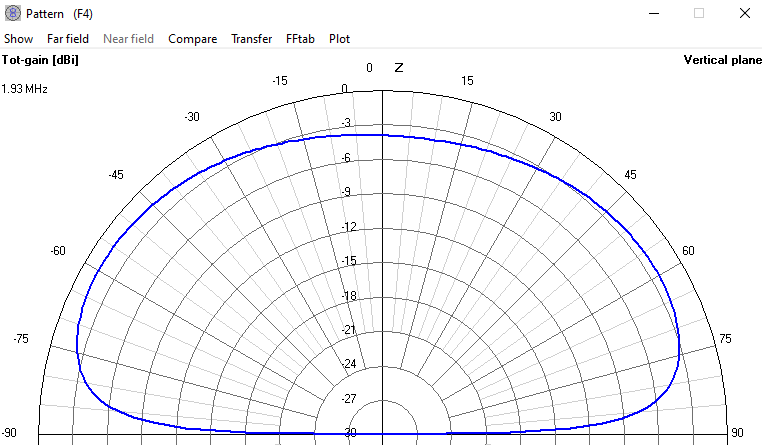
Figure 7 – Extended Inverted L Vertical Radiation Pattern
Comparing the real antenna and the NEC2 simulation, the real antenna presented a feed impedance of 24 Ω measured with an MFJ 259B antenna analyser. The calculated figure was 22.7 Ω.
Extended ‘Further’ Inverted L (Antenna 6) – Tried and Tested
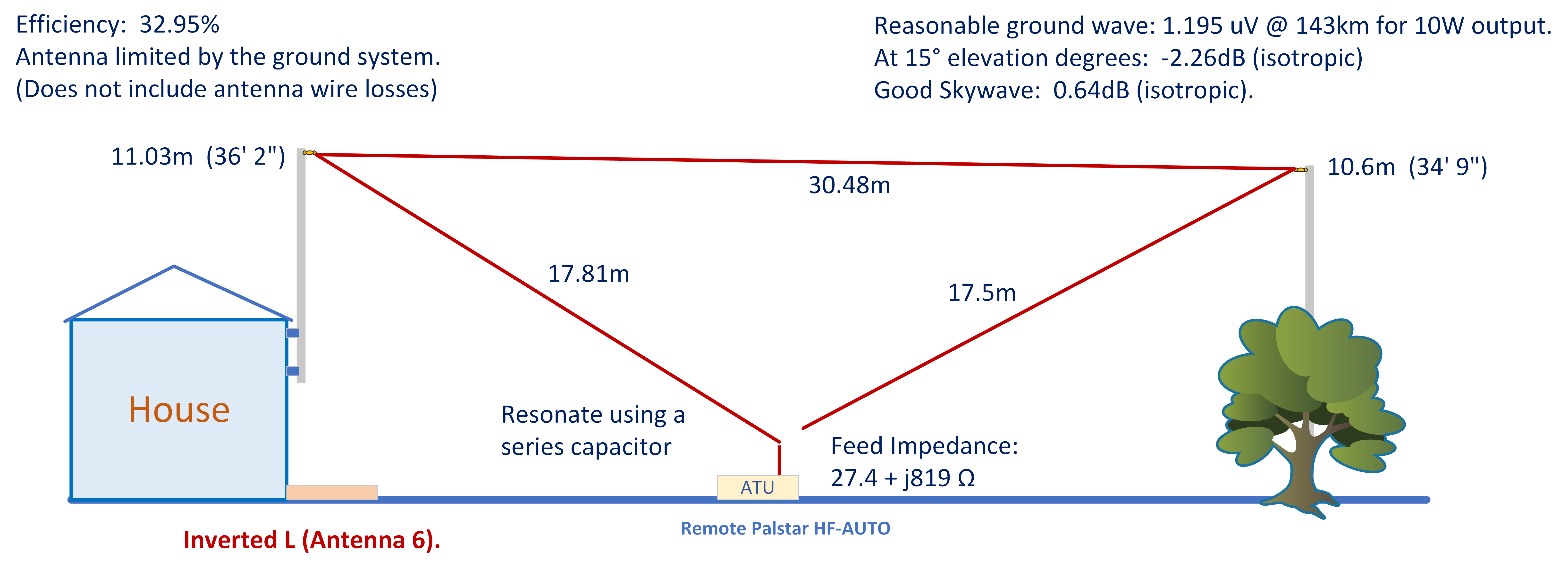
This antenna is 65.8 m (216 ft) long which is getting close to a halfwave. However, the resistive feed impedance worked out at only 27.4 Ω which is not very convenient. The associated inductive reactance was j819 Ω that is easily tuned using a series capacitor.
If the antenna is extended slightly to around 67.8 m, the extra length increased the feed impedance to around 50 + j1230 Ω. In fact, a simulation of the extended antenna (By adding 3 m in length) resulted in an input impedance that varied between (23.3 + j753) Ω and (90 + j1724) Ω from 1.8 MHz to 2.0 MHz respectively. It means that the antenna length can be trimmed to find 50 Ω at any frequency in the band. I cancelled the inductive reactance using a series capacitor of approximately 68 pF. This eliminating the need for a tuning unit. Note that some interaction takes place when the antenna is tuned – the resistive elements changes slightly when resonance is achieved. It means that the final trimming must be done using an antenna impedance meter.
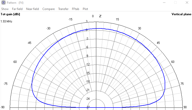
Figure 8 – Extended ‘Further’ Inverted L Vertical Radiation Pattern
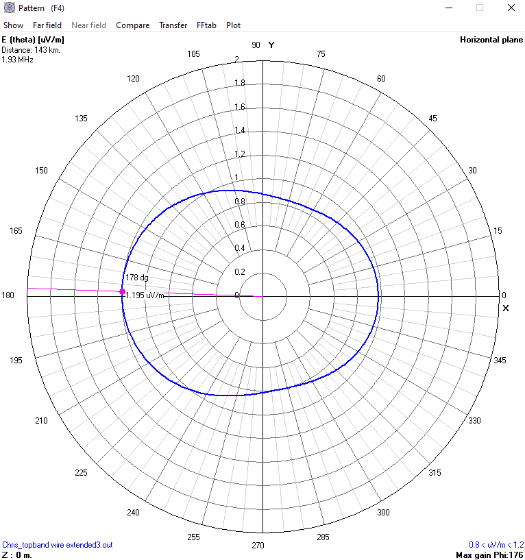
Figure 9 – Extended ‘Further’ Inverted L Horizontal Surface Wave Pattern at 143 km
The main disadvantage of this arrangement is the voltage rating of the series capacitor. A transmitter delivering 1 kW generates a peak voltage of around 7,800 V across the 68 pF capacitor! That’s a rather extreme case but the message here is – be aware. It is best to avoid flashing-over an expensive ATU.
This antenna increased the NVIS by 4.56 dB. It is not surprising; the current maxima now occurred in the horizontal part of the antenna approximately 40 m from the end. Figure 9 shows that the horizontal radiation pattern at 143 km is distorted reducing propagation in some directions slightly. However, maximum ground wave remains reasonable. I noted that a local web-SDR station showed a signal reduction of 3 dB compared to the simple L antenna labelled as ‘Antenna 4’. It seems that if you get increased NVIS then you have to pay the piper in some other way.
With the 68 pF series capacitor deployed and tuned for resonance at 1.93 MHz, the antenna was tried on the other HF bands using the Palstar HF-Auto ATU. All bands matched apart from 80 m. Of course, the HF-Auto was not needed on 160 m.
Inverted Delta Loop (Antenna 7) – Tried and Tested – Failure
This antenna turned out to be a mixed bag. The theoretical efficiency was the highest of the practical antennas at 40.83%. However, no matter how much I tried, I could not get it to tune using the dimensions shown.
NEC2 predicted that the halfwave resonance of the loop should occur around 2.4 MHz. That appears correct if you think of the antenna as a shorted quarter wave stub of length approximately 32.9 m. A quarter wave of 32.9 m corresponds roughly to a resonance at 2.29 MHz.
The theoretical feed impedance is 47.2 + j3268 Ω at 1930 kHz and requires only a tiny capacitor typically 25 pF to tune it. It should be obvious from the capacitor size that it will not tune. Connecting the loop to the feeder cable via a balun and series capacitor detunes the antenna because of stray capacitance. The resonance of the loop drops to a frequency well below 1.8 MHz. The antenna simply will not tune without introducing series inductance. The losses associated with the inductor would devastate the efficiency. For this reason, I cannot recommend it.
The detail above is the theoretical results from NEC2. Figure 10 shows the attempted and failed method of feeding the antenna.
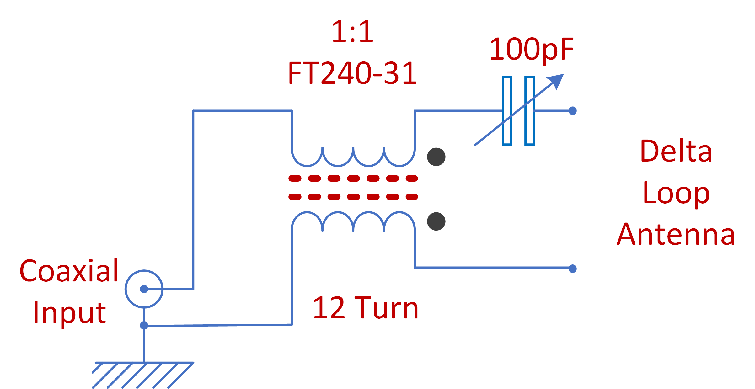
Figure 10 – Delta Loop Feed Method – Failed
Just for completeness, I included the theoretical antenna patterns of the delta loop below.
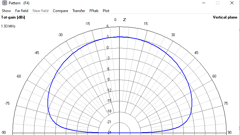
Figure 11 – Delta Loop Vertical Radiation Pattern
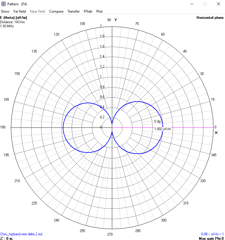
Figure 12 – Delta Loop Horizontal Radiation Pattern
Just as a side note: I connected the inverted delta loop directly to the HF-Auto without a balun and without a series tuning capacitance. This configuration tuned well (but it was probably not efficient). One side of the loop connected to the ATU unbalanced output and the other end connected to the case of the ATU, that is connected to RF Earth. Using this configuration on WSPR with 20 W on 1836 kHz during April 2020, I received a spot from the Neumayer Station in Antarctica which is a hop of approximately 13,748 km. An impressive hop. However, I still cannot recommend it!
Inverted Delta Loop in Common Mode (Antenna 8) – Tried and Tested
Although the inverted delta loop was a failure (at least the version shown above and simulated in NEC2), I did wonder if the additional wire length and capacitance of the wire to ground could provide a vertical with natural quarter wave resonance. This could be that low-loss dream suburban antenna? The answer is no!
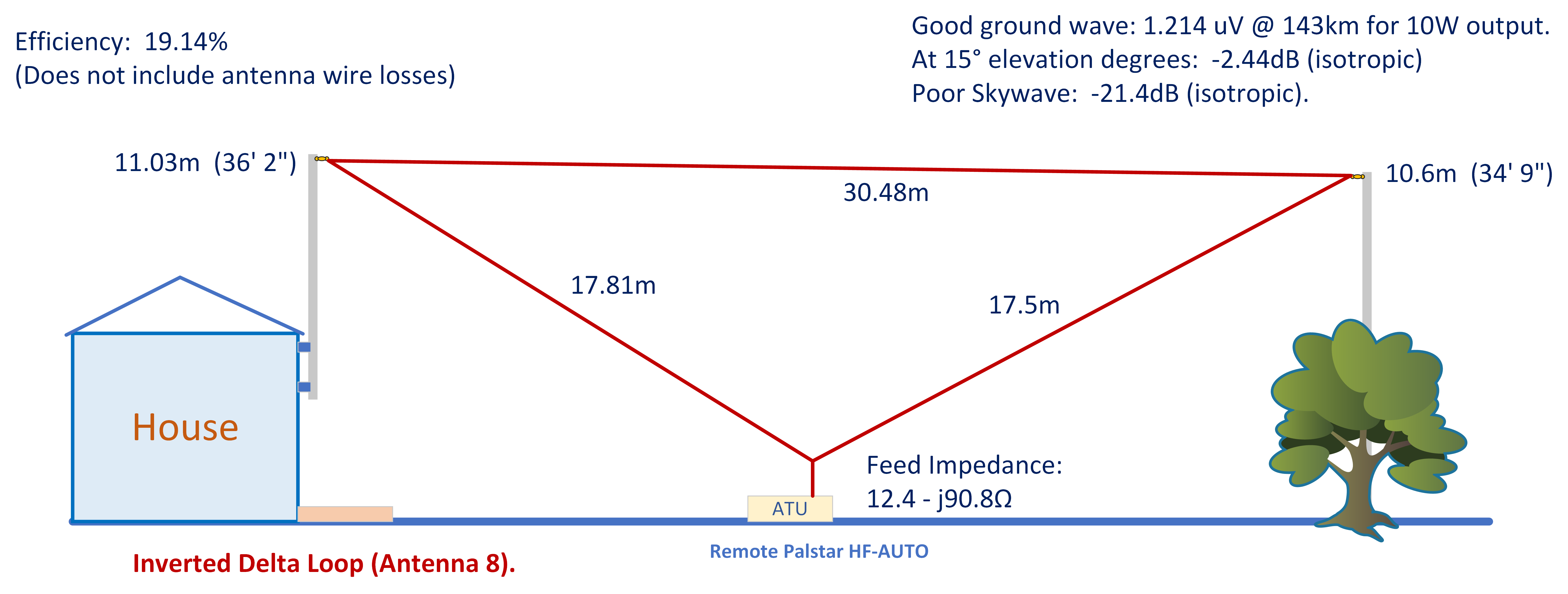
Energising the whole loop as one element is quite interesting. The feed impedance is low of course and the antenna efficiency drops to about 19%, which is as expected.
Figure 13 – Delta Loop CM Horizontal Radiation Pattern
NEC2 predicted the reactive part of the antenna impedance as -j90.8 Ω capacitive. This is slightly lower than the -j192 Ω offered by the common-mode fed G5RV antenna (See Antenna 13). Presumably, the extra wire in the delta loop presented more capacitance to earth requiring less inductance to achieve quarter-wave resonance. The difference between the CM connected inverted delta loop and the CM connected G5RV is minimal. Losses in the antenna wire resistance and the loading coil will probably reduce efficiency to below 19%. Thick wire and a heavy-duty loading coil could help here.
Figure 13 shows the 10 W ground wave at 143 km. The radiation pattern is essentially circular and reaches 1.214 μV/m. That level of signal just about moves the ‘S’ meter on the WEB-SDR. A daytime SSB contact at that distance is probably possible but it would be a struggle.
Half wave Dipole (Antennas 9, 10, 11 and 12) – Fantasy Antenna
Many strong stations on topband employ a horizontal or inverted ‘V’ halfwave dipole. It seems prudent to include this in the investigation as a comparison even though the practical installation at many suburban sites is difficult or impossible.
To demonstrate the practical issues, the following diagram shows the antenna size relative to the size of the plot at my QTH. At a push, the dipole ends could be bend into convoluted shapes to fit it into the garden. Lowering the dipole ends to ground level, for example by running it along the top of a fence, would probably reduce efficiency considerably. This was not tried but it is a possibility.
Interestingly, the NEC2 simulated halfwave (at 38 ft) seemed better for NVIS than the other antennas. The halfwave figure is +4.3 dB relative to an isotropic source. Even better is the halfwave at 60 ft; that gave a theoretical NVIS figure of 6.35 dB. This is conformation of a fact that most people already know: A halfwave dipole is probably the best 160 m antenna for night time inter ‘G’ nattering over a few hundred miles.
Another interesting fact shown up by NEC2 is that the dipoles perform more efficiently without the earth mat.
Figure 15 – Dipole at 38 Ft – Horizontal Radiation Pattern
Presumably, the earth mat is too short. The disadvantage of the dipole is the relatively poor surface wave and the mediocre radiation at lower angles. Figure 15 shows the horizontal surface wave for the dipole at a height of 38 ft. Deep nulls at 90° and 270° limits the effectiveness.
The ideal situation is a 60 ft halfwave dipole (or higher) used as a dipole for night time nattering. For DX or local ground wave working, the antenna could be fed in common mode by strapping feeders and loading it against earth (obvious really). However, this is a fantasy antenna for me so I cannot get excited.
G5RV (Antenna 13) – Tried and Tested
The final antenna investigated here is the G5RV dipole or 102 ft doublet. This antenna is so common on the bands that I felt obliged to include it. In practice, the top length of 102 ft fitted exactly between the masts and it is easy to match on all bands. I admit to running this antenna for a couple of years. On topband, the feeders must be strapped and the whole antenna fed against earth as a top-loaded vertical. The centre of the antenna droops alarmingly even with light-weight feeders.
Figure 16 – NEC2 Representation of the G5RV and Earth Radial System
The common mode performance of the G5RV is similar to the delta loop (when fed in common mode). If anything, this antenna is slightly better but there is no method of adapting it to create NVIS. If an attempt is made to feed the dipole in differential mode on 160 m the results are hopeless – it is just too short and does not work efficiently. My HF-Auto failed to find a match.
In fact, this antenna is not particularly efficiently on 80 m either despite the large number of people who claim otherwise. The feed impedance measured on the end of the ladder line on my antenna measured only 5 + j91 Ω @ 3.6 MHz. This forces the use of an ATU. In my case, if I run 400 W output, the ladder line feels warm to the touch. A load of 5 Ω (after tuning) suggests currents on the ladder line around 8.9 A. No wonder it heats up! The May 2014 QST test review of the Palstar HF-AUTO ATU revealed a power loss of 19% on 80 m if the antenna impedance drops to around 6 Ω. That works out at approximately 1.8 dB loss. The combined feeder and ATU losses are significant.
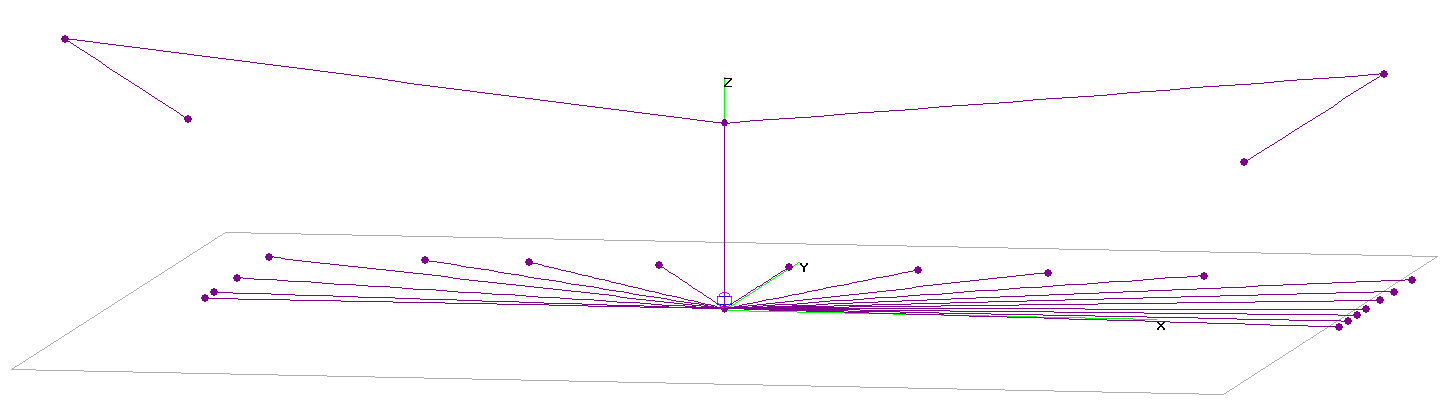
Figure 17 – NEC2 Representation of the G5RV and Earth Radial System with Tails
The final variation is a modified G5RV that employs 5 m tails on the ends of the top section. The idea was to maximise the RF current in the vertical element of the antenna and make it more efficient. However, the reverse is true. The tails reduced efficiency, reduced radiation at 15° elevation and reduced surface waves along the ground. I don’t really understand why this happened. I can only guess that reducing the height of the voltage maxima (the antenna ends) increased the loss above lossy ground. Another failure!
A general antenna rule for long wires is: keep the voltage maxima well away from the ground.
Conclusions
I cannot help think that I have reinvented the wheel. Most of the conclusions reported here are things most amateurs already know instinctively. However, converting wives-tales into hard facts is difficult and involved a lot of messing around in the shack and garden. For me this has been fun and I have learnt a few tricks that makes it worthwhile. The conclusions are:
- The antenna and earth system must be complementary. There is no point building massive antenna structures if the earth mat you employ is inadequate. Even the theoretical quarter‑wave vertical performed disappointingly in this case.
- Depressingly, the performance of a 160 m station is pre-determined by the quality of the soil/land that surrounds it. If the antenna is above the sea then any antenna, no matter how crap, will probably work well. Conversely, if you live above gravel then you have a serious challenge if you want to work DX!
- Earth rods just don’t work in ‘average’ soil. I found they made no detectable difference at all.
- Raised earth radial systems appear more efficient than buried systems.
- An inverted delta loop close to half-wave resonance promised high efficiency but proved impossible to feed.
- Watch out for low impedance feed points if you use an ATU. Yes, they will tune nicely but the losses can be huge even with big tuners like the HF-Auto. It is better to use a series capacitor to tune the antenna and a balun to step up the impedance to 50 Ω.
- Avoid inductors if you can – they always introduce series loss.
- Keep high voltage parts of the antenna away from the ground. Don’t let the ends of wires droop to ground level.
- Within the limits of a given QTH, you can maximise for low angle using verticals or maximise NVIS using Horizontals but not both. Antennas with mixed polarity tend to be mediocre. An example of this is the inverted ‘L’.
- There appears to be a rule that states: The radial lengths must be at least as long as the height of the vertical. This needs more investigation but I am not sure how!
- It is a struggle to achieve much more than 20% efficiency with a pure vertical antenna on 160m. Although NEC2 reported the 60 ft vertical as 25%, the loading coil losses would diminish that figure significantly.
73 Chris