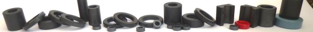
Many radio amateurs employ antenna analysers. These provide a quick and easy way to measure impedance. Most analysers work on the same principle. A digital or free running VFO drives a load via a directional coupler or bridge. The instrument measures the RF incident and reflected signal voltages using a rectifier and an A/D converter. The onboard processor calculates and displays the required results.
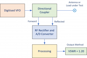
Figure 1 – Outline of a Typical Antenna Analyser
These devices work great for day-to-day measurements where quick look-see results suffice. However, they share a common problem. The measurement of high or low impedance, well removed from 50Ω, results in poor accuracy.
I often use the MFJ-259 for quick measurement. For more serious results, my preference is the ‘SDR-Kits’ Vector Network Analyser V3 (which I think is excellent for the price) – See Figure 2.
The VNA V3 software performs single port measurements (S11) similar to the MFJ-259. However, the main advantage is the ability to perform accurate insertion loss measurements between the two ports and display complex S21 data.
Strictly speaking S11, S21 and the reflection coefficient ‘p’ are power ratios. However, it is useful to define them in terms of voltage ratio. Using the definition in Wikipedia for a two-port network:
The 2-port S-parameters have the following generic descriptions:
S11 is the input port voltage reflection coefficient.
S12 is the reverse voltage gain.
S21 is the forward voltage gain.
S22 is the output port voltage reflection coefficient.
Definition S11
S11: This is defined as the voltage ratio of the signal reflected at the input port to the incident signal. Strictly speaking this is with the output of the network terminated by a matched load.
Hence, in a two-port network, S11 and the reflection coefficient (ρ) are essentially the same.
Definition S21
S21: This is the ratio of the voltage signal measured at the output port to the signal measured at the input port.
S11 and S21 results are nearly always complex numbers. The magnitudes of the real and imaginary parts are always less than 1.0 For example, a possible S11 result could be: S11 = 0.356 +j 0.217 (where ‘j’ is a complex operator)
The Problem
A problem arises if you make a direct impedance measurement using the S11 method. For example, by connecting an impedance directly across the ‘TX Out’ connector. This results in a graph calibrated directly in ohms. However, we must remember that the instrument actually measures the reflection coefficient ‘ρ’ and not impedance.
The reflection coefficient ρ, is defined as:
where is always 50Ω and
is the wanted impedance. Rearranging for
:
It is easy to assume that this result is accurate but often it is not. To illustrate the problem let
Now increase by say 1% so that
. The corresponding impedance is calculated as
an increase of 9,949% Even a tiny error in
, possibly due to the directional coupler, can translate into very large errors in
. A similar case exists with very low impedance values. Here the reflection coefficient is negative. For example, if
, then
. You can apply the same logic as above and find similar errors.
Results suggest that the S11 method of impedance measurement is only satisfactory over a limited range of impedance magnitudes typically 4Ω to 650Ω. This range corresponds to S11 values of approximately -0.86 and +0.86 respectively. I noticed that the MFJ-259 reports impedance modulus above 650 Ohm as R(Z)650> suggesting that MFJ are aware of the limitations and avoid misleading the user – which is commendable. I should point out that S11 is always complex so stating a value of +0.86 is a little simplistic.
The second problem relates to how the reflection coefficient behaves with complex loads at higher frequencies. Restating equation 1:
In most cases the load is complex. Consider a resistor ‘R’ in series with an inductor ‘L’ and assume they are ideal components. Then:
where
Substitute this into equation 1:
As the frequency increases, increases as does
. Eventually a frequency is reached where:
and so
This implies, at high frequencies, that the reactance dominates over the resistive component particularly when R is low.
tends towards 1.0 for inductive loads. Similarly, for a capacitor and resistor in parallel (for example a resistor with lead capacitance), then:
which tends to zero as increases. Hence, in this case, when substituted in equation 1:
In other words, as the frequency increases, the reactive components swamp the restive parts of the load and the reflection coefficient rapidly approaches +1.0 for inductive loads and -1 for capacitive loads. This is exactly the region of where massive uncertainty occurs!
S11 impedance measurements are ok at low frequencies but suspect elsewhere. Another question is: why do we need to measure high impedance at RF? For me, I want to measure the common mode impedance of my balun. The MFJ-259 will not read above 650Ω and does not tell me if the reactance is capacitive or inductive!
Solution (For High Z Measurements)
A better method of measuring a series impedance is to place the required impedance in the transmission path of a vector network analyser and then measure the forward transmission loss and then calculate
.
This method is very useful for measuring balanced loads. The output port and input port of the VNA are both terminated in a precision 50Ω load.
The following is a derivation of the correction factors required to calculate impedance from S21 measurements. For high impedance measurements, place the impedance in series with the two ports and measure the forward transmission. The series impedance is calculated as:

Derivation:
These calculations must employ complex arithmetic throughout. The first part is a calibration process. With the output and input ports connected together, the output voltage is:
Following insertion of the series impedance, the output voltage drops to:
Taking the ratio of the two voltages, then by definition:
Rearranging and solving for :
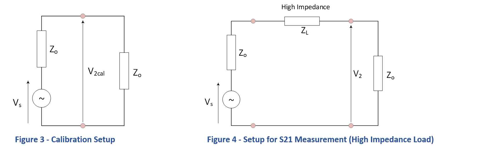
Solution (For Low Z measurements)
Unless you are measuring very low antenna impedance at LF or you are attempting to measure the impedance of a resonant magnetic loop directly (?) there is probably no need to use the following correction. However, I include it for completeness.
For a low impedance load circuit, the principle of measurement is almost identical. In this case, the load impedance is placed in parallel with the input port (Rx in). In the same way, measure the forward transmission and then calculate
.
The load impedance is calculated as:

The derivation is as follows:
Without the load impedance, with the output and input ports joined together, the output voltage is the same as before. From Figure 3:
Following insertion of the parallel impedance, the output voltage drops:
Taking the ratio of the two voltages:
Rearranging and solving for :
This correction may be useful for loads below 1Ω or even lower than 0.1 Ω. It would be necessary to minimise lead inductance to an absolute minimum and use a purpose-built jig.
Setup – Measure S11 and S21
To test these ideas, I measured three ¼ Watt 1% metal film resistors at frequencies up to 100MHz. Surface mount components perform better at RF and are the better choice of component. However, this is a rough and ready demonstration and not a serious implementation.
Resistor values tried were: 1kΩ, 10kΩ and 22kΩ. The test set-up employed a measurement jig constructed from tin-plated circuit board and two BNC chassis mounted sockets. These connected to the Network Analyser using adaptors.
To calibrate the S11 port, I temporarily removed the calibration jig and connected open-circuit and short-circuit elements on adapters as per usual. An attempt was made to align the RF length of the adapters during calibration with the RF length used for measurement.
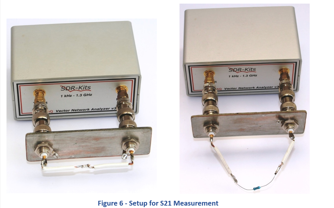
Similarly, Figure 6 shows the method for measuring S21. The resistor lead length remained the same during the S11 and S21 methods. This is all a bit crude but good enough at low frequencies. For this reason, I only measured to 100MHz and I take results above 30 MHz with a large pinch of salt!
At RF, a Metal Film resistor with leads presents resistance, inductance and capacitance typically as shown in Figure 7.

It means that the impedance plots will exhibit complex behaviour as the frequency rises. It also implies that the impedance modulus of the resistor will probably fall with frequency. However, even simple circuit are full of surprises so it is best not to guess.
Convert S21 into S11
Not surprisingly, most network analysers include a means to implement mathematical manipulation of data. For example, the VNA v3 includes a built-in function that converts S21 into Ohms automatically and displays the results on a graph without any user effort. As a bonus, there is no need to know anything about manipulating complex numbers.
The expression
converts S21 into S11. In other words, it converts transmission loss into a reflection coefficient. Once the results are in S11 form, the standard software displays the impedance in real, imaginary, modulus or whatever form you want including Smith Charts.
You may be wondering where does this correction comes from?
This is derived from Equations 2 and 3.
and
Equating to eliminate :
After a tidy up and some messing around
Using the Corrected S21 Method to Estimate the Common Mode Impedance of a Current Balun
Measuring a resistor is fine but a more interesting target is real antenna hardware. This example is a current balun that I built for 160m and HF. It consists of 15 turns of RG58 coax wound on a Fair-Rite FT240-31 core. I guessed at the number of turns so it will be interesting to see if it works. Figure 8 shows the test setup.
S21 measurements were recorded and converted by equation 5 to determine S11. Figure 9 shows results for Resistance, Reactance and Modulus all in Ohms.
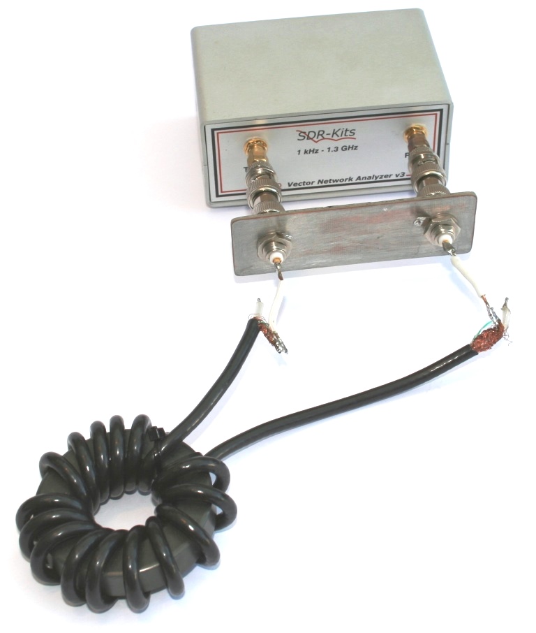
Figure 8 – FT240-31 Balun Test – Setup
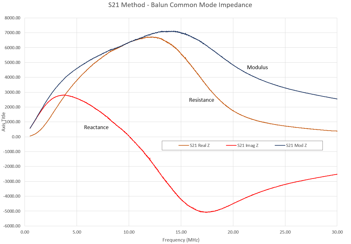
Figure 9 – FT240-31 Balun Performance (S21 Method)
The results are good. The balun provides approximately 1000 Ohms of resistive loss from 2 to 22 MHz. The reason for including the balun measurement, is to demonstrate the difference between the S21 and S11 impedance measurement methods. The S21 method is based on a theoretical model and, in my opinion, provided the best chance of seeing a reasonable version of the truth under these conditions. Any kind of impedance measurement at RF is thwart with difficulty.
As a comparison, Figure 10 shows the results for the FT240-31 balun using the S11 impedance measurement method.
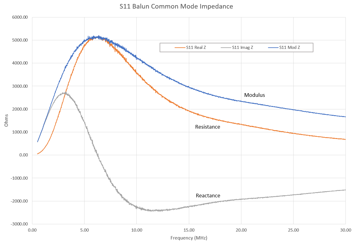
Figure 10 – FT240-31 Balun Performance (S11 Method)
Figure 11 is a comparison of the impedance magnitude for the S11 and S21 methods. We should remember that this is a measure of the same balun and the two results should be the same! It is clear that at higher frequencies the impedance modulus is heading towards zero implying that lead capacitance is taking precedence.
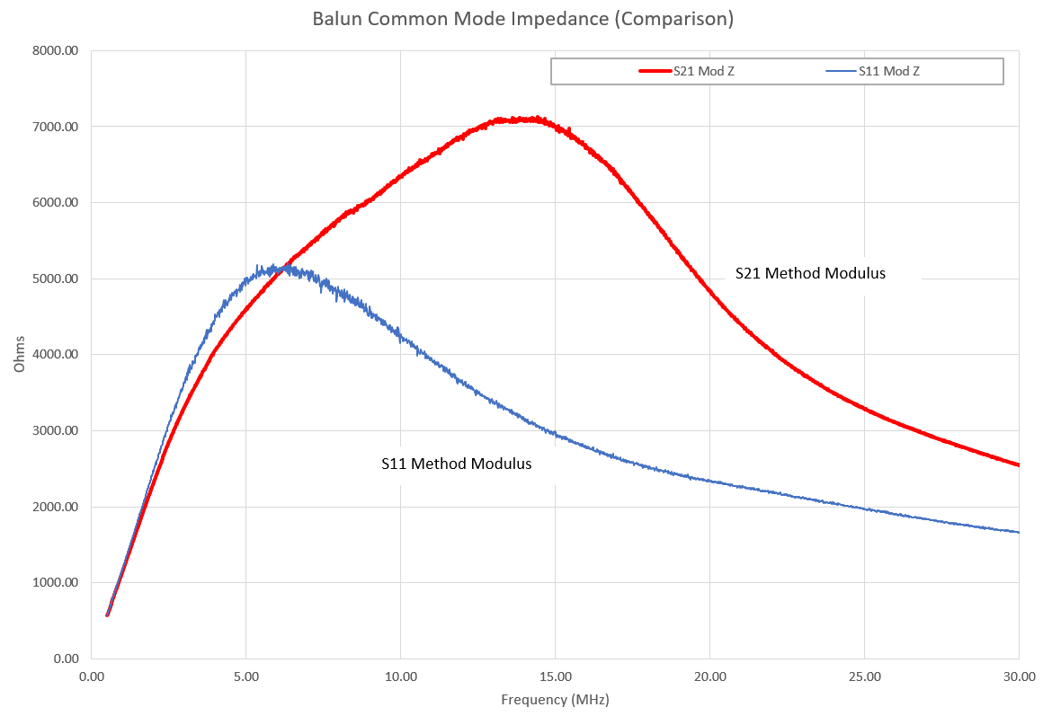
Figure 11 – FT240-31 Balun – Comparison of Modulus
Results from Measuring Resistors
This section illustrates a few results from measuring resistors. To keep things simple, I have plotted only the modulus of the impedance. If you want more details, I suggest trying it for yourself.
Figure 12 illustrates impedance modulus results for a 22kΩ resistor. The two plots represent measurement using S21 corrected by Equation 5 and direct results applying the S11 method. The difference between the two plots is significant and shows the limitation of the S11 method. The results using S21 are as expected – a gradual HF role off.
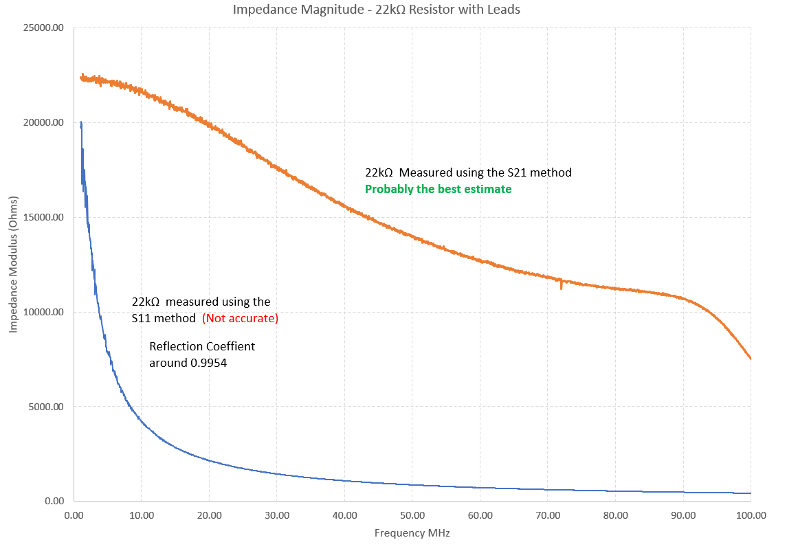
Figure 12 – Results For a 22KΩ Resistor
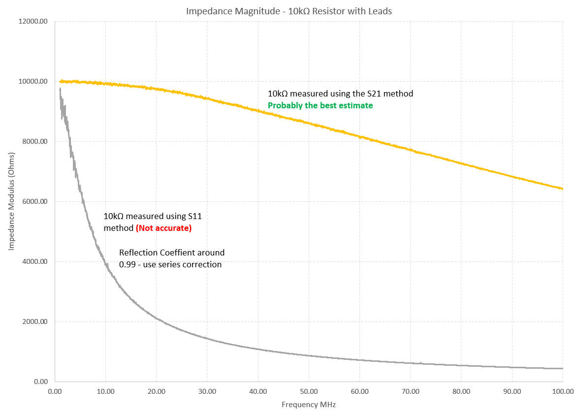
Figure 13 – Results For a 10KΩ Resistor
The trend seems apparent. As the resistor value fall lower in value the S21 and S11 results converge. Once the impedance is down to about 650Ω then you may as well use the S11 method. Figure 13 and Figure 14 shows plots for 10kΩ and 1 kΩ resistor respectively.
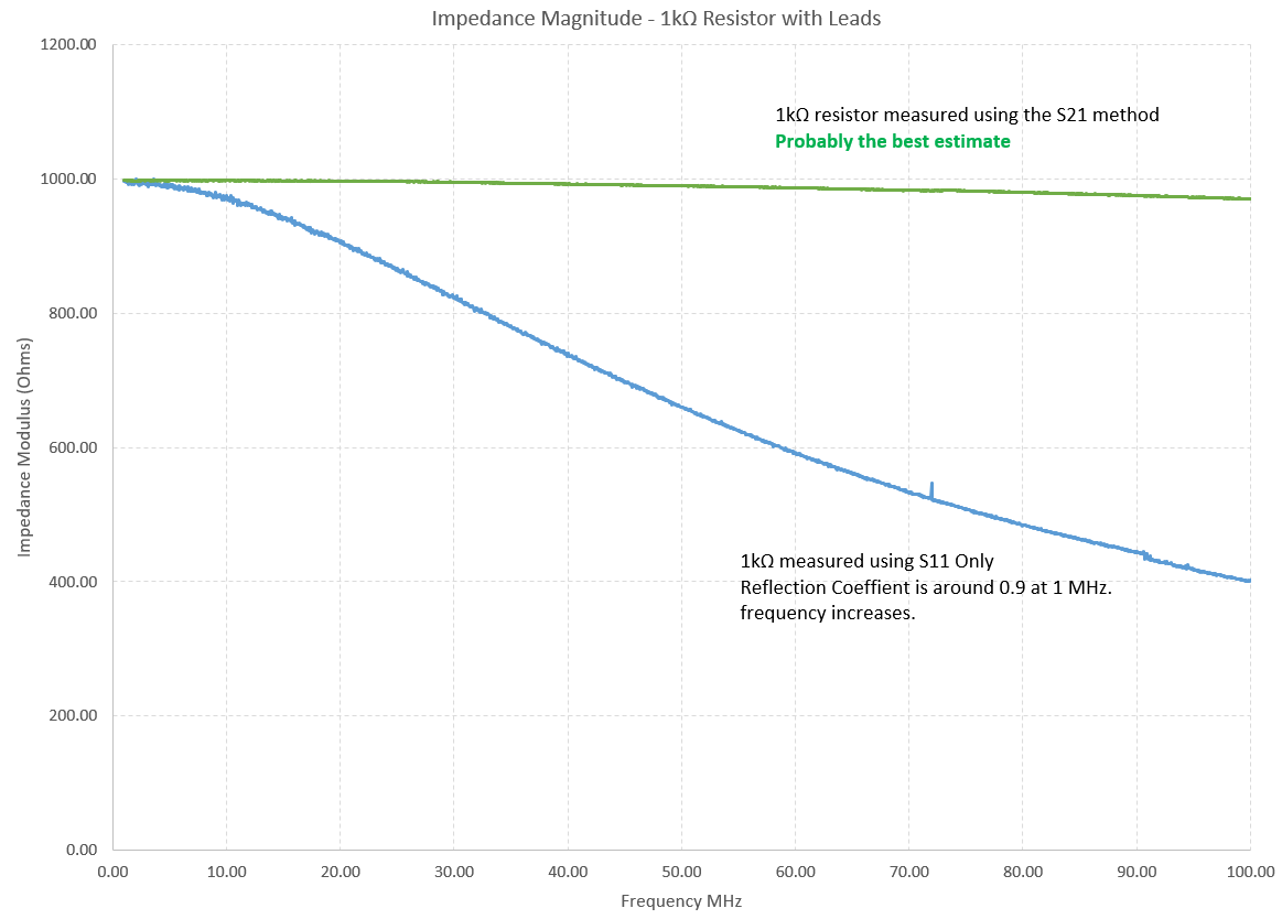
Figure 14 – Results For a 1KΩ Resistor
The problem with any RF measurement, other than those confined to a strictly controlled 50Ω system, is that you never know if you are correct – how do you check it? Hence, I will not make any generalised conclusions other than to say that the S21 measurement method is another tool in the box but be careful how you use it.
Keep on measuring
73 Chris